
Welcome
Database Management System
Course: COMP 163
Time: 08:00 AM - 09:15 AM on Monday, Wednesday, Friday
Location: John T Chambers Technology Center 114 (CTC 114)
| Week | Topic | Assignment (Canvas + GitHub) | Database | Comment |
|---|---|---|---|---|
| 1 (Jan 12, Jan 14, Jan 16) | Introduction to Database Management System | Lab 1 + Homework 1 (2w) | SQLite | |
| 2 (Jan 21, Jan 23) | Entity Relationship Model | Holiday on Monday (Jan 19) | ||
| 3 (Jan 26, Jan 28, Jan 30) | Relational Algebra | Lab 2 + Homework 2 (2w) | ||
| 4 (Feb 2, Feb 4, Feb 6) | Relational Database Interfaces | PostgreSQL | ||
| 5 (Feb 9, Feb 11, Feb 13) | Relational Database Advanced SQL | Lab 3 + Homework 3 (2w) | ||
| 6 (Feb 18, Feb 20) | Relational Database Normalization | Project Part 1 (4w) | Holiday on Monday (Feb 16) | |
| 7 (Feb 23, Feb 25, Feb 27) | Relational Database Table Indexing | MariaDB | ||
| 8 (Mar 2, 4, 6) | Midterm Preparation | Midterm (Mar 6) | ||
| 9 (–) | Spring Break | |||
| 10 (Mar 16, 18, 20) | Relational Database Transactions | Lab 4 + Homework 4 (2w), Project Part 2 (4w) | OracleSQL | |
| 11 (Mar 23, 25, 27) | Relational Database Security | |||
| 12 (Mar 30, Apr 1, 3) | Relational Database and Data Distribution | Lab 5 + Homework 5 (2w) | ||
| 13 (Apr 6, 8, 10) | Relational Database and Data Aggregation | ClickHouse | ||
| 14 (Apr 13, 15, 17) | Relational Database and NoSQL, Semester Review | Final Preparation | ||
| 15 (Apr 20, 22, 24) | Project Presentation (15 min) | |||
| 16 (Apr 27) | Project Presentation (15 min) | Classes End (April 28) | ||
| 17 (May 4) | Final Exam: Monday, May 4th, 10-11 AM |
Module 1
Introduction to Database Management Systems
Agenda
- Start Module 1
- Review Topics
- Review Syllabus
What is a Database?
- A database is an organized place to store data
- Built for large amounts of data
- Built to keep data consistent over time
- Data is stored so it can be found again later
Database: Store → Find
Database as Storage
- A database is an organized place to store data
- Data is structured
- Storage is intentional, not ad hoc
Flower
------
id: 101
name: "Rose"
color: "Red"
price: 2.50
Large Amounts of Data
- Databases handle large volumes of data
- Much more than what fits in memory
- Designed to grow over time
Flowers
-------
101 | Rose    | Red    | 2.50
102 | Tulip   | Yellow | 1.75
103 | Lily    | White  | 3.00
104 | Daisy   | White  | 1.25
105 | Orchid  | Purple | 4.50
...
(Thousands of rows)
Consistency Over Time
- Databases keep data consistent
- Rules prevent invalid entries
- Same data seen by all users
Rule:
price >= 0

✔ Rose   | 2.50
✔ Tulip  | 1.75
✘ Lily   | -3.00  ← rejected
Finding Data Again
- Data is stored so it can be found again later
- Queries let us ask questions
- Results are predictable and repeatable
SELECT name, price
FROM flowers
WHERE color = 'White';

Result:
Lily  | 3.00
Daisy | 1.25
Why a Database Management System (DBMS)?
What is a DBMS?
- A DBMS is software that manages a database
- It sits between applications and stored data
- Applications do not access data files directly
App / Website / API / Software
              ↓
   --------- DBMS ---------
              ↓
    Database (disk / SSD)
Databases Before DBMS
| System | How it Stores Data | How you Query | Main Problem |
|---|---|---|---|
| Paper | Handwritten records | Search by reading | Slow, hard to scale |
| Files (folders) | Documents in directories | Manual naming + search | Duplicates, inconsistent versions |
| Spreadsheets | Rows and columns | Filters and formulas | Hard for multi user + rules |
| Custom App (ad hoc) | Program specific format | Whatever the app supports | No standard, hard to maintain |

Problem: Duplication → Inconsistency
Before 1900: Manual Systems
- Before 1440 – Manual Writing: Handwritten records
- 1440 – Printing Press: Faster copying
- 1800s – Shipping Letters: ~10–14 days by ship

Edgar F. Codd
- Born: August 19, 1923
- Known for: Relational Database Model
- Key Contribution: Relational Algebra, Normal Forms
- Impact: Foundation of SQL and modern databases
- Award: ACM Turing Award (1981)

20th Century: The Digital Revolution
- 1970 – Relational Database
- 1980s – SQL: Standard query language
- 1990s – Client Server: Multi user databases
- 2000s – Digitalization: Paper to databases

21st Century: Connectivity and Real-Time Revolution
- Cloud: Scalable remote databases
- Big Data: Massive data processing
- AI: Smarter data analysis
- Edge: Low latency storage

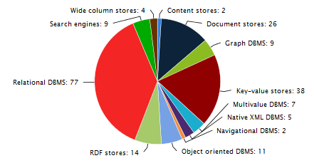
Types of Databases
| Type | Data Shape | Good For | Example |
|---|---|---|---|
| Relational | Tables (rows/columns) | Business data, consistency | PostgreSQL, MySQL |
| Document | JSON like documents | Flexible fields, web apps | MongoDB |
| Key Value | Key → value | Caching, sessions | Redis |
| Column Store | Columns (analytics) | Fast aggregates | ClickHouse |
| Graph | Nodes + edges | Relationships, networks | Neo4j |
- Relational is our main focus
- Others exist for different data and workloads
- Same goal: store and query data
Choose by Data Shape
Why a Database Management System 🤔
- Many devices produce data continuously
- Many users need shared access
- Many apps depend on the same source of truth
- Apps read and write data
- APIs connect services
- DBMS keeps data consistent
- Transactions ensure correct updates
- Concurrency control supports many users at once
- Constraints prevent invalid data
- Indexes improve query performance
- Security rules control who can access what
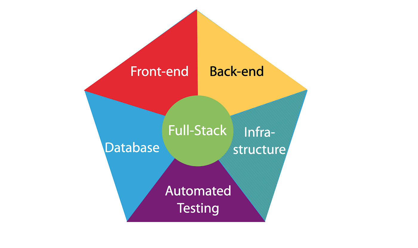
Three Core Components of a Software System
Each component has a distinct role, but all three must work together.
LLMs and SQL: Human Review Still Required
- LLMs can generate SQL, results are not always correct
- Generated queries may:
- use invalid syntax
- reference the wrong tables or columns
- misinterpret the intent of the question
- Incorrect SQL can:
- return misleading results
- update the wrong rows
- delete data permanently
-- Generated by an LLM
DELETE FROM orders;

-- Missing WHERE clause
-- Result: all rows deleted
Conclusion: LLMs can assist, but humans must review SQL before execution.
What Skill Changes
- Software evolves quickly
- Frameworks change every few years
- Languages rise and fall
- Tools are frequently replaced
- Hardware evolves rapidly
- Faster CPUs and storage
- New architectures and platforms
- Short upgrade cycles
- Data lasts much longer than software
- Databases persist across generations of technology
- Applications are rewritten, but data remains
- Good database design protects long-term value
Why a Relational Database Management System?
- Tables match how we organize records
- SQL gives a standard interface
- Constraints protect correctness
- Transactions protect consistency
Relational DBMS: Core Pieces
Relational Model: The Idea
- Entity → a table
- Row → a record
- Key → identity + links
flowers(id, name, color, price)
orders(id, flowerId, qty)
| StudentId | Name | Major |
|---|---|---|
| 101 | Ana | CS |
| 102 | Ben | EE |
| 103 | Cam | CS |
Keys Connect Tables
Agenda
- Review Module 1 (DBMS foundations)
- CREATE: database and table structure
- SQLite dialect and file based model
- SQLite data types and type affinity
- Flower domain schema design
- Preview: installation and coding
Question
SELECT name, price
FROM flowers
WHERE price > 2.00;
Can this query be used in programs written in Java, C++, and Python?
- No, SQL queries are specific to Java
- Each program requires a different query syntax
- Yes, but only if the database is SQLite
- Yes, SQL is programming language
Answer (click)
Show answer
Correct: D
SQL is a database query language. The same SQL query can be sent from Java, C++, Python, or any other language through a database API.
Java
Connection conn = DriverManager.getConnection(url);
Statement stmt = conn.createStatement();
ResultSet rs = stmt.executeQuery("""
SELECT name, price
FROM flowers
WHERE price > 2.00
""");
Python
conn = sqlite3.connect("flowers.db")
cur = conn.cursor()
cur.execute("""
SELECT name, price
FROM flowers
WHERE price > 2.00
""")
C++
sqlite3* db;
sqlite3_open("flowers.db", &db);
sqlite3_exec(db,
"SELECT name, price FROM flowers WHERE price > 2.00",
nullptr, nullptr, nullptr);
JavaScript
const db = new sqlite3.Database("flowers.db");
db.all(
`SELECT name, price
 FROM flowers
 WHERE price > 2.00`, callback);
Question
Which component is executing the SQL query?
- The programming language runtime
- The operating system
- The database managment system
- The text editor used to write the query
Answer (click)
Show answer
Correct: C
The DBMS parses, plans, and executes SQL. Programming languages only send the query and receive results.
PROGRAM
Java · Python · C++ · JS

send SQL string
DBMS
parse
plan
execute
DATABASE
flowers.db

tables
rows
indexes
Question
What is the role of a programming language when working with a database?
- To replace SQL entirely
- To store data directly on disk
- To send SQL commands to the DBMS
- To define how tables are physically stored
Answer (click)
Show answer
Correct: C
Applications use programming languages to communicate with the DBMS, but SQL remains the interface for data access.
Imperative
# step-by-step instructions
# how to do it

for flower in flowers:
  if flower.price > 2.00:
    print(flower.name, flower.price)
- Tell the computer how
- Explicit steps
- Order matters
Declarative
-- describe the result
-- what you want

SELECT name, price
FROM flowers
WHERE price > 2.00;
- Tell the DBMS what
- DBMS decides how
- SQL is descriptive
Query A:
SELECT * FROM flowers;

Query B:
INSERT INTO flowers(name, price)
VALUES ('Rose', 2.50);
- Does the order of these queries matter?
- Would the result be the same if we swap them?
Show answer
- Yes, sometimes order matters
- If queries depend on earlier changes
- Read-only operations are not affected by order
- SQL is descriptive, but execution order still matters
From Concepts to Structure
- So far: what databases and DBMSs are
- Now: how structure is defined
- Focus today is CREATE, not querying
What Does CREATE Mean?
- CREATE defines structure
- No data is stored yet
- It defines tables, columns, and rules
Database vs Table (SQLite)
- Database: one file (
.db) - Table: structure inside the file
- SQLite has no server process
flowers.db
 ├─ flowers
 ├─ suppliers
 └─ orders
PROGRAM
Java · Python · C++ · JS

send SQL string
DBMS
parse
plan
execute
DATABASE
flowers.db

tables
rows
indexes
CLI
sqlite3 flowers.db

enter SQL
SQLite as a SQL Dialect
- SQLite follows standard SQL closely
- Some syntax differences exist
- Most important difference: typing model
SQLite Type System
- SQLite uses dynamic typing
- Columns have type affinity
- Values decide their type at runtime
Five Core SQLite Data Types
| Type | Description | Flower Example |
|---|---|---|
| INTEGER | Whole numbers | flower_id |
| REAL | Decimal numbers | price |
| TEXT | Strings | name, color |
| BLOB | Binary data | image |
| NULL | Missing value | unknown_color |
Flower Domain
- Simple and familiar example
- Focus on structure, not complexity
- Used consistently across examples
Flower Table: Logical Design
flowers(
  id,
  name,
  color,
  price
)
Choosing SQLite Data Types
| Column | Type | Reason |
|---|---|---|
| id | INTEGER | Primary identifier |
| name | TEXT | Flower name |
| color | TEXT | Readable attribute |
| price | REAL | Decimal value |
CREATE TABLE (Preview)
CREATE TABLE flowers (
  id INTEGER PRIMARY KEY,
  name TEXT,
  color TEXT,
  price REAL
);
Constraints Still Matter
- Flexible typing does not mean no rules
- Constraints protect data quality
price REAL CHECK (price >= 0)
What We Are Not Doing Yet
- No INSERT
- No SELECT
- Structure comes first
Next: Installing SQLite
- sqlite3 command line tool
- Verify installation
- Create first database file
Then: Hands On SQL
- Create tables
- Insert flower data
- Run simple queries
Summary
- CREATE defines structure
- SQLite uses type affinity
- Good design still matters
Agenda
- Concept: Database and Schema
- SQLite data types
- Designing a flower database
- Preparing for installation and coding
What Does CREATE Mean?
- CREATE defines structure, not data
- It tells the DBMS what tables look like
- No rows yet, only rules
Database vs Table
- Database: container (file in SQLite)
- Table: structured collection of rows
- SQLite database = single
.dbfile
flowers.db
 ├─ flowers
 ├─ suppliers
 └─ orders
SQLite Is File Based
- No server to start
- No username or password by default
- Database is a file you can copy
SQLite Dialect of SQL
- SQLite supports most standard SQL
- Some differences from MySQL / PostgreSQL
- Flexible typing (important!)
SQLite Type System
- SQLite uses dynamic typing
- Columns have an affinity, not a strict type
- Values decide their type at runtime
Five Core SQLite Data Types
| Type | Description | Flower Example |
|---|---|---|
| INTEGER | Whole numbers | flower_id |
| REAL | Decimal numbers | price |
| TEXT | Strings | name, color |
| BLOB | Binary data | image |
| NULL | Missing value | unknown_color |
Type Affinity in SQLite
- INTEGER, TEXT, REAL are preferred
- SQLite does not strictly enforce types
- Design discipline matters
Flower Domain
- We model a simple flower shop
- Flowers, prices, colors, stock
- Simple and familiar domain
Flower Table: First Design
flowers(
  id,
  name,
  color,
  price
)
Choosing Data Types
| Column | Type | Reason |
|---|---|---|
| id | INTEGER | Unique identifier |
| name | TEXT | Flower name |
| color | TEXT | Human readable |
| price | REAL | Decimal value |
CREATE TABLE (Preview)
CREATE TABLE flowers (
  id INTEGER PRIMARY KEY,
  name TEXT,
  color TEXT,
  price REAL
);
Primary Key in SQLite
INTEGER PRIMARY KEYis special- Aliases the internal rowid
- Auto increments by default
Constraints Matter
- Even with flexible typing
- Rules protect data quality
price REAL CHECK (price >= 0)
What We Are NOT Doing Yet
- No inserts
- No queries
- Focus is structure
Next: Installing SQLite
- sqlite3 command line tool
- Verify installation
- Create first database file
Then: Hands On Coding
- Create tables
- Insert flower data
- Run simple queries
Summary
- CREATE defines structure
- SQLite uses flexible typing
- Good design still matters
Case Study: Furniture Store Inventory (SQLite)
- Goal: Draft each query
- After each step: run a SELECT to verify
- Then: new requirement → ALTER TABLE → verify again
Step 1: Create the Table
- Create a table named
inventory - Columns:
idINTEGER PRIMARY KEYnameTEXT NOT NULLcategoryTEXT NOT NULLpriceREAL NOT NULLquantityINTEGER NOT NULL
Show answer
CREATE TABLE inventory (
  id INTEGER PRIMARY KEY,
  name TEXT NOT NULL,
  category TEXT NOT NULL,
  price REAL NOT NULL,
  quantity INTEGER NOT NULL
);
Verify 1
- Verify the table exists and columns are correct
- Use a SQLite CLI command (not SQL)
Show answer
.schema inventory
Step 2: Insert Data
- Insert three rows:
- Oak Table, Table, 299.99, 4
- Leather Sofa, Sofa, 899.00, 2
- Desk Lamp, Lamp, 39.50, 12
- Write three INSERT statements
Show answer
INSERT INTO inventory (name, category, price, quantity)
VALUES ('Oak Table', 'Table', 299.99, 4);

INSERT INTO inventory (name, category, price, quantity)
VALUES ('Leather Sofa', 'Sofa', 899.00, 2);

INSERT INTO inventory (name, category, price, quantity)
VALUES ('Desk Lamp', 'Lamp', 39.50, 12);
Verify 2
- Read the inventory table
- Show: id, name, category, price, quantity
Show answer
SELECT id, name, category, price, quantity
FROM inventory;
Business Question
- List items with low stock
- Definition: quantity <= 3
- Return: name, quantity
Show answer
SELECT name, quantity
FROM inventory
WHERE quantity <= 3;
New Requirement
- The store now needs to track the supplier for each item
- Add a new column:
supplier(TEXT) - Then fill it for existing rows
Step 3: ALTER TABLE
- Add a new column
suppliertoinventory - Type: TEXT
Show answer
ALTER TABLE inventory
ADD COLUMN supplier TEXT;
Verify 3
- Verify the new column exists
- Use a SQLite CLI command
Show answer
.schema inventory
Step 4: Update Existing Rows
- Set supplier values:
- Oak Table → Pacific Furnishings
- Leather Sofa → West Coast Leather
- Desk Lamp → BrightHome
- Write three UPDATE statements
Show answer
UPDATE inventory
SET supplier = 'Pacific Furnishings'
WHERE name = 'Oak Table';

UPDATE inventory
SET supplier = 'West Coast Leather'
WHERE name = 'Leather Sofa';

UPDATE inventory
SET supplier = 'BrightHome'
WHERE name = 'Desk Lamp';
Verify 4
- Read and confirm supplier values
- Return: id, name, supplier, quantity
Show answer
SELECT id, name, supplier, quantity
FROM inventory;
Final Check
- List all items supplied by BrightHome
- Return: name, category, quantity
Show answer
SELECT name, category, quantity
FROM inventory
WHERE supplier = 'BrightHome';
Agenda
- Primary key
- Constraints:
UNIQUE,NOT NULL,DEFAULT - Relationships: foreign keys
- Lab 1 overview
- Homework 1 overview
Primary Key
First the concept, then the SQL (using our Furniture Store case study).
Definition (No Meaning)
- A primary key is a column (or columns) to identify rows
- It is an identifier only (no semantic meaning required)
- It exists so rows can be referenced precisely
inventory
---------
id | name         | category | price  | quantity
1  | Oak Table    | Table    | 299.99 | 4
2  | Leather Sofa | Sofa     | 899.00 | 2
3  | Desk Lamp    | Lamp     | 39.50  | 12
Row Identity
What a Primary Key Enforces
- Uniqueness (no duplicates)
- Stability (used for references)
- One row ↔ one key value
Good:
id = 1, 2, 3, 4, ...

Bad:
id = 1, 1, 2, 3  (duplicate)
Why We Need It
- Target exactly one row
- Avoid accidental multi-row updates
- Enable relationships later (foreign keys)
Without a key:
UPDATE inventory
SET price = 10
WHERE category = 'Lamp';

Could affect many rows.
Primary Key in Our Case Study
- Table:
inventory - Primary key:
id - Chosen as a simple numeric identifier
id is not "meaningful".
It is just an identifier.

name/category can change
id should not.
SQL: Defining the Primary Key
CREATE TABLE inventory (
  id INTEGER PRIMARY KEY,
  name TEXT NOT NULL,
  category TEXT NOT NULL,
  price REAL NOT NULL,
  quantity INTEGER NOT NULL
);
SQLite: Auto-Generated IDs
INTEGER PRIMARY KEYcan be auto-generated- You can omit
idduring INSERT - SQLite assigns a new integer value
INSERT INTO inventory (name, category, price, quantity)
VALUES ('Oak Table', 'Table', 299.99, 4);

-- id assigned automatically
AUTOINCREMENT (When to Use)
- For stricter "never reuse old ids" behavior
- Prevents reusing a deleted id later
- Usually not needed, but good to know
id INTEGER PRIMARY KEY AUTOINCREMENT
SQL: Primary Key with AUTOINCREMENT
CREATE TABLE inventory (
  id INTEGER PRIMARY KEY AUTOINCREMENT,
  name TEXT NOT NULL,
  category TEXT NOT NULL,
  price REAL NOT NULL,
  quantity INTEGER NOT NULL
);
SQLite will keep increasing id values even if rows are deleted.
ID Generation Concept
Verify the ID Was Assigned
- Always run a SELECT after inserts
- Confirm rows and IDs match expectations
SELECT id, name, category, price, quantity
FROM inventory;
Safe Updates Use the Key
- Primary key targets one row
- Reduces risk of mass updates
- More reliable than matching on names
UPDATE inventory
SET price = 279.99
WHERE id = 1;
Safe Deletes Use the Key
- Primary key targets one row
- Prevents deleting multiple matches
- Use with care
DELETE FROM inventory
WHERE id = 1;
Key Takeaway
Primary keys exist for correctness and control.
Constraints
Rules enforced by the database to protect data quality.
Common Constraints
- NOT NULL : value must exist
- UNIQUE : no duplicates allowed
- DEFAULT : value assigned automatically
price REAL NOT NULL
sku TEXT UNIQUE
quantity INTEGER DEFAULT 0
NOT NULL
Prevents missing critical information.
- Column must always have a value
- INSERT fails if value is missing
- Useful for required attributes
name TEXT NOT NULL,
category TEXT NOT NULL,
price REAL NOT NULL
UNIQUE
Prevents duplicate values across rows.
- Ensures values do not repeat
- Often used for identifiers
- Different from primary key
sku TEXT UNIQUE
DEFAULT
Provides a value when none is supplied.
- Reduces required input
- Prevents NULL values
- Encodes common assumptions
quantity INTEGER DEFAULT 0
Updated Inventory Table
CREATE TABLE inventory (
  id INTEGER PRIMARY KEY AUTOINCREMENT,
  name TEXT NOT NULL,
  category TEXT NOT NULL,
  sku TEXT UNIQUE,
  price REAL NOT NULL,
  quantity INTEGER DEFAULT 0
);
Why Constraints Matter
- Catch errors early
- Protect data integrity
- Reduce application complexity
Relationships Between Tables
Real systems connect data across tables.
Inventory and Suppliers
Foreign Key Example: Referencing Values
Supplier Table (Parent)
| id (PK) | name | country |
|---|---|---|
| 1 | Pacific Furnishings | USA |
| 2 | West Coast Leather | USA |
| 3 | BrightHome | Canada |
Inventory Table (Child)
| id (PK) | name | category | supplier_id (FK) |
|---|---|---|---|
| 101 | Oak Table | Table | 1 |
| 102 | Leather Sofa | Sofa | 2 |
| 103 | Desk Lamp | Lamp | 3 |
Example: Supplier and Inventory Relationship
Each inventory item references exactly one supplier using a foreign key.
name = "Pacific Furnishings"
references supplier.id
name = "Oak Table"
supplier_id = 1
The database enforces that supplier_id = 1 must exist in the
supplier table before the inventory row can be inserted.
Foreign Key
A reference to a primary key in another table.
- Links rows across tables
- Preserves consistency
- Prevents invalid references
supplier_id INTEGER
REFERENCES supplier(id)
Create Supplier Table
CREATE TABLE supplier (
  id INTEGER PRIMARY KEY AUTOINCREMENT,
  name TEXT NOT NULL,
  contact_email TEXT UNIQUE
);
Link Inventory to Supplier
CREATE TABLE inventory (
  id INTEGER PRIMARY KEY AUTOINCREMENT,
  name TEXT NOT NULL,
  category TEXT NOT NULL,
  price REAL NOT NULL,
  quantity INTEGER DEFAULT 0,
  supplier_id INTEGER,
  FOREIGN KEY (supplier_id)
    REFERENCES supplier(id)
);
What the Foreign Key Enforces
- Supplier must exist before assignment
- No orphan records
- Clear ownership relationships
Key Relationships Summary
Takeaway
Constraints and keys are not optional. They are the foundation of reliable, maintainable databases.
Case Study Extension
The furniture store now wants to manage suppliers separately.
New Requirement
- Each item is supplied by exactly one supplier
- A supplier can provide many inventory items
- Supplier information must be stored only once
New Entity: Supplier
- Track supplier identity and contact information
- Enforce data quality using constraints
- Prepare for relationships with inventory
Task 1: Design the Supplier Table
- Table name:
supplier - At least 3 attributes
- Include a primary key
- Use NOT NULL and UNIQUE where appropriate
Think about what uniquely identifies a supplier and what information should never be missing.
Suggested Attributes
id: unique supplier identifiername: supplier nameemail: contact emailphone: optional contact number
Task 2: Create the Supplier Table
- Use
INTEGER PRIMARY KEY AUTOINCREMENT - Ensure
nameis NOT NULL - Ensure
emailis UNIQUE
Show example
CREATE TABLE supplier (
  id INTEGER PRIMARY KEY AUTOINCREMENT,
  name TEXT NOT NULL,
  email TEXT UNIQUE NOT NULL,
  phone TEXT
);
Verify the Supplier Table
- Use a SQLite shell command
- Confirm columns and constraints
.schema supplier
Relationship Requirement
- Each inventory item references one supplier
- This is a one-to-many relationship
- Implemented using a foreign key
Inventory–Supplier Relationship
Task 3: Add Supplier Reference
- Add
supplier_idto inventory - Use a foreign key constraint
- Reference
supplier(id)
In SQLite, foreign keys must be enabled explicitly.
SQLite Foreign Key Reminder
PRAGMA foreign_keys = ON;
Run this before creating or using foreign key constraints.
Updated Inventory Table (With Supplier)
CREATE TABLE inventory (
  id INTEGER PRIMARY KEY AUTOINCREMENT,
  name TEXT NOT NULL,
  category TEXT NOT NULL,
  price REAL NOT NULL,
  quantity INTEGER DEFAULT 0,
  supplier_id INTEGER NOT NULL,
  FOREIGN KEY (supplier_id)
    REFERENCES supplier(id)
);
What This Prevents
- Assigning non-existent suppliers
- Duplicate supplier data
- Inconsistent relationships
Checkpoint
You now have: entities, primary keys, constraints, and a foreign key relationship enforced by SQLite.
Lab 1: Library Database
Due: January 30, 11:59 PM
Goal: model, design, and implement a small relational database from a real-world
scenario.
Problem Scenario
A local library wants to track books loaned to members.
- Members can borrow multiple books
- Each book is borrowed by only one member at a time
- Library staff manage the loans
Step 1: Identify Entities
Entities are the things the system needs to track.
- Look for nouns in the scenario
- Ignore vague or irrelevant objects
- Each entity represents a table later
Entity Examples (Correct vs Incorrect)
| Good Entities | Bad Entities |
|---|---|
| Book | City |
| Member | Chair |
| Staff | Building |
Step 2: Identify Relationships
Relationships describe how entities are connected.
- Who borrows what?
- Who manages which action?
- Think in verbs, not nouns
Step 3: Create a UML-based ERD
- Use PlantUML to define entities
- Each entity needs at least 3 attributes
- Include a primary key
- Add data types and constraints
Output: libraryERD.png
ERD Structure Reminder
@startuml
entity "Book" {
  +book_id : INTEGER
  title : TEXT
  isbn : TEXT
}

entity "Member" {
  +member_id : INTEGER
  name : TEXT
  email : TEXT
}

Book -- Member : borrows
@enduml
Step 4: Create Tables in SQLite
- Translate ERD into CREATE TABLE statements
- Use PRIMARY KEY and FOREIGN KEY
- Apply NOT NULL and UNIQUE where needed
Verify using the .schema command
Step 5: Perform CRUD Operations
| Operation | What You Do |
|---|---|
| Create | INSERT at least 3 rows |
| Read | SELECT all rows |
| Update | Change a value in one row |
| Delete | Remove one specific row |
What to Submit
- libraryERD.png – UML diagram
- librarySchema.png – SQLite .schema output
- libraryCrud.png – CRUD operation screenshots
This lab connects concepts → design → SQL implementation.
Homework 1: SQL Foundations
Due: January 30, 11:59 PM
Focus: conceptual understanding of SQL, SQLite, and course expectations.
Purpose of This Homework
This homework ensures you understand the role of SQL, the difference between language and system, and the scope of the course.
- No advanced syntax required
- Focus on ideas, not memorization
- Your own words matter
Required Reading
Please read Chapters 1 and 2 of the following books:
- SQL: The Complete Reference
- The Definitive Guide to SQLite
Goal: general understanding, not mastery of syntax.
Reading Guidance
- What problem does SQL solve?
- What role does a DBMS play?
- How data is created, queried, and changed
Do not worry about remembering every command.
Homework Questions (Conceptual)
- Why is SQL important?
- What is the difference between SQL and SQLite?
Answer in your own words. Short, clear explanations are preferred.
SQL Keywords to Explain
Explain the purpose of each keyword:
CREATESELECTUPDATEDELETEINSERT
What We Are Looking For
- What each keyword does conceptually
- When it is used
- No complex SQL examples required
Precision of thought matters more than syntax.
Syllabus Acknowledgment
Please read the course syllabus carefully:
- List any questions or points of clarification
Why the Syllabus Matters
- Defines course structure and expectations
- Explains grading and policies
- Clarifies responsibilities on both sides
Submitting this homework confirms that you reviewed the syllabus.
Submission Summary
- Answer all questions clearly
- Use your own words
- Submit via Canvas
This homework sets the foundation for everything that follows.
Module 2
Entity Relationship Model (ERM)
Agenda
- Requirements → entities
- Entities and relationships
- Cardinality: 1:1, 1:N, N:N
- Attributes, data types, constraints
- ERD → SQL schema
-- Work order:
-- 1) requirements
-- 2) ERD
-- 3) SQL schema
-- 4) queries
Every Database Management System Starts with
Requirements
Requirement
The system should allow users to rent bikes easily
Requirement
The system should allow registered users to rent a bike by selecting a location, choosing an available bike, and completing payment through the application within three steps
Requirement
Purpose: Bike Rental Database System to manage rentals and track customers, bikes, and transactions
- Track availability of bikes, including unique id, condition, and location
- Log rental transactions, including bike id, customer id, start time, return time
- Maintain customer records, including name, contact details, rental history
Translate Requirements → Model
- Underline nouns → candidate entities
- Underline verbs → candidate relationships
- Details become attributes
-- Nouns: user, bike, location, payment, transaction
-- Verbs: rent, select, choose, pay
-- Candidate entities:
--  - Customer
--  - Bike
--  - Location
--  - Payment
-- - RentalTransactionEntities
- Real world objects or concepts
- Usually nouns
- Later implemented as tables
-- Entity candidates:
-- Customer
-- Bike
-- RentalTransaction
-- Location
-- Payment
Relationships
- Connections between entities
- Usually verbs
- Shown as lines in ERD
-- Relationship examples:
-- Customer rents Bike
-- Bike located at Location
-- Customer pays Payment
Quick Check
- Question: "Customer rents a Bike"
- Is it an entity or a relationship?
-- ERD view:
-- Customer  --(rents)-->  Bike
Quick Check
- Question: "Bike"
- Is it an entity or a relationship?
-- Entity will have attributes:
-- BikeID, Model, Color, Condition, Availability
Name Rules
- Conceptually, ERD names can overlap
- Technically, table names must be unique
- Use consistent casing
-- Prefer consistent names:
-- Customer, Bike, RentalTransaction
-- Avoid reserved words for table names
Case Sensitivity
- Conceptually, case does not matter in ERD
- Technically, it depends on DB and OS
-- Safe habit:
-- Pick a naming style and keep it.
-- Example: PascalCase tables, snake_case columns
Requirement
A travel booking system should allow users to search for, compare, and book flights, hotels, and rental cars. Users must be able to filter results by price, date, and location, and securely complete payments
Requirement (highlight nouns/verbs)
A travel booking system should allow users to search for, compare, and book flights, hotels, and rental cars. Users must be able to filter results by price, date, and location, and securely complete payments.
Text → Visual
- Text is good for brainstorming
- ERD is good for precision and review
- ERD is easier to validate as a group
-- Practice:
-- turn nouns into entity boxes
-- connect boxes with verb labels- Conceptual model of the database
- Shows entities and their attributes
- Illustrates relationships between entities
- Independent of any database system

Attributes
- Entities are not enough
- Each entity has a list of attributes
- Attributes become columns
-- Customer attributes:
-- CustomerID, Name, Email, Phone

-- Bike attributes:
-- BikeID, Model, Color, Condition, Availability
Primary Key Attribute
- Mandatory technical attribute
- Unique per row
- Often integer
-- Primary key examples:
-- Customer(CustomerID)
-- Bike(BikeID)
-- RentalTransaction(RentalID)- Each entity includes a primary key
- Primary key uniquely identifies each record
- Primary key cannot be NULL
- Primary key remains stable over time

Optional Attributes
- Extra details keeps the system useful
- Not needed to identify the entity
- Often nullable
-- Optional examples:
-- Customer.Email, Customer.Phone
-- Bike.Color, Bike.Condition
-- RentalTransaction.ReturnDate- Entities can have multiple descriptive attributes
- Attributes store detailed information
- Not all attributes are required for identification
- Attributes refine the meaning of an entity

Data Types
- Each attribute has a data type
- Data types impact validation and storage
- Keep types aligned across layers
-- BookingDate DATE
-- Availability BOOLEAN
-- Name VARCHAR(100)- Each attribute is assigned a data type
- Data types define how values are stored
- Correct types prevent invalid data
- Data types must align with application logic

SQL Standard Data Types
| Data Type | Description | Example |
|---|---|---|
| INTEGER | A whole number, no decimal points | 42 |
| BIGINT | A large integer value | 9223372036854775807 |
| DECIMAL(p, s) | Exact numeric value | DECIMAL(10, 2) |
| FLOAT | Approximate numeric value | 3.14159 |
| CHAR(n) | Fixed length string | CHAR(5) |
| VARCHAR(n) | Variable length string | VARCHAR(50) |
| TEXT | Variable length text | "long notes" |
| DATE | Date | 2025-01-14 |
| TIME | Time | 14:30:00 |
| TIMESTAMP | Date and time | 2025-01-14 14:30:00 |
| BOOLEAN | TRUE or FALSE | TRUE |
| BLOB | Binary data | [bytes] |
Constraints
- Rules that protect the database
- Improve correctness
- Make errors visible early
-- Common constraints:
-- PRIMARY KEY
-- FOREIGN KEY
-- NOT NULL
-- UNIQUE
-- DEFAULT- Constraints enforce data correctness
- Primary keys ensure uniqueness
- NOT NULL prevents missing values
- UNIQUE avoids duplicate data

SQL Attribute Constraints
| Constraint | Description |
|---|---|
| PRIMARY KEY | Uniquely identifies each record; implies NOT NULL |
| FOREIGN KEY | Ensures referential integrity by linking to another table |
| NOT NULL | Column cannot be NULL |
| UNIQUE | All values in a column are distinct |
| DEFAULT | Default value when no value is provided |
| AUTO_INCREMENT | Auto generates unique integer id (DB specific) |
Conceptual vs Technical (SQL) Terms
| Conceptual Term | Technical Term |
|---|---|
| Diagram | Schema |
| Entity | Table |
| Attribute | Column |
| Record | Row |
| Identifier | Primary Key |
| Relationship | Foreign Key |
| Optional Attribute | Nullable Column |
| Mandatory Attribute | NOT NULL Column |
From ERD to Database Schema
CREATE TABLE Customer (
  CustomerID INTEGER PRIMARY KEY AUTOINCREMENT,
  Name VARCHAR(100) NOT NULL,
  Email VARCHAR(100) UNIQUE,
  Phone VARCHAR(15)
);

CREATE TABLE Bike (
  BikeID INTEGER PRIMARY KEY AUTOINCREMENT,
  Model VARCHAR(100) NOT NULL,
  Color VARCHAR(50),
  Condition VARCHAR(50),
  Availability BOOLEAN DEFAULT TRUE
);

CREATE TABLE RentalTransaction (
  RentalID INTEGER PRIMARY KEY AUTOINCREMENT,
  CustomerID INTEGER NOT NULL,
  BikeID INTEGER NOT NULL,
  BookingDate DATE NOT NULL,
  ReturnDate DATE,
  FOREIGN KEY (CustomerID) REFERENCES Customer(CustomerID),
  FOREIGN KEY (BikeID) REFERENCES Bike(BikeID)
);
Misaligned Data Types
- Same data, different types across layers
- Causes validation failures and data loss
- DB rejects invalid formats
-- Example risk:
-- UI collects phone as text "+1-123-456"
-- DB column INTEGER
-- Insert fails or loses formatting
Examples of Misaligned Data Types
| Front-End | Back-End | Database | Result |
|---|---|---|---|
| Text input for phone number | String validation for format | INTEGER type | Formatted numbers rejected |
| Dropdown allows decimal selection | Expects integer values | FLOAT type | Unexpected decimal input |
| Date picker with local format | Assumes ISO format | DATE type | Date conversion errors |
ERD Quiz (1/3)
- Question: What does an entity represent?
- A. A database table
- B. A real world object or concept
- C. A relationship between tables
- D. A data attribute
-- Entity → table later
-- Example: Customer, Bike
ERD Quiz (2/3)
- Question: What is the purpose of a relationship?
- A. To store data
- B. To define data types
- C. To show how entities connect
- D. To create unique identifiers
-- Relationship example:
-- Customer rents Bike
ERD Quiz (3/3)
- Question: What is the purpose of a primary key?
- A. Allow duplicate rows
- B. Uniquely identify each row
- C. Establish relationships
- D. Enforce data types
-- Primary key column:
-- CustomerID INTEGER PRIMARY KEY
How to Model Relationships in ERD?
Cardinality matters: 1:1, 1:N, N:N
1 Entity
0 Relationship

2 Entity
1 Relationship

3 Entity
2 Relationship

- Travel booking application domain
- Users search and compare options
- Bookings include flights, hotels, and rental cars
- Attributes capture price, date, and location

Why Minimum Relationships?
- Performance: less joins
- Simplicity: easier to maintain
- Clarity: easier to explain and test
- Consistency: less places for mismatch
-- Design tip:
-- prefer the simplest ERD that meets requirements
-- add complexity only when needed
Relationship Types (Cardinality)
| Cardinality | Meaning | Example |
|---|---|---|
| 1:1 | Each record links to one record | User and Profile |
| 1:N | One record links to many records | Customer and Rentals |
| N:N | Many records link to many records | Students and Courses |
When to Use Relationship Type?
| Cardinality | When to Use | Example |
|---|---|---|
| 1:1 | Each record in one table corresponds to exactly one record in another table | User and Profile |
| 1:N | One record can be associated with multiple records in another table | Library and Books |
| N:N | Multiple records in both tables can be related to each other | Students and Courses |
Querying Relationships
- One relationship → one join
- More relationships → more joins
- Start from the filtering table
SELECT Book.title
FROM Book
WHERE Book.isbnId = '978-1-';

SELECT Book.title
FROM Book, ISBN
WHERE Book.bookId = ISBN.bookId
  AND ISBN.isbnId = '978-1-';

SELECT Book.title
FROM Book, ISBN, Book_ISBN
WHERE Book.bookId = Book_ISBN.bookId
  AND ISBN.isbnId = Book_ISBN.isbnId
  AND ISBN.isbnId = '978-1-';
Which Relationship?
| # | Scenario | Which Cardinality? |
|---|---|---|
| 1 | Book and ISBN | |
| 2 | Author and Book | |
| 3 | Student and borrow Book | |
| 4 | Student and Student ID | |
| 5 | Book and Publisher | |
| 6 | Publisher and Books | |
| 7 | Library and Book | |
| 8 | Book and Format (e.g., eBook, hardcover) | |
| 9 | Book and Catalog Number in the Library System | |
| 10 | Reader and Book Review |
Module 2 Recap
- Requirements drive the model
- Entities (nouns) become tables
- Relationships (verbs) connect entities
- Attributes need types and constraints
- ERD becomes SQL schema
-- Next step:
-- use your ERD to justify every CREATE TABLE line- Draft an ERD for a bike rental store
- Identify core entities (e.g., Bike, Customer, Rental)
- List key attributes for each entity
- Mark primary key attributes
- Decide which entities are connected
@startuml
entity "EntityA" as A {
  +id : INTEGER
  attribute_1 : VARCHAR
  attribute_2 : INTEGER
}

entity "EntityB" as B {
  +id : INTEGER
  attribute_1 : VARCHAR
}

A -- B : "relationship"
@enduml
Case Study
Furniture Store Database
Requirements → ERM → Tables → Data
Agenda
- Gather requirements
- Extract entities and relationships
- Build ERM (PlantUML)
- Convert to SQL tables
- Insert sample data
- Query and maintain data
-- Work order:
-- 1) requirements
-- 2) ERM / ERD
-- 3) schema
-- 4) data
-- 5) queriesRequirement
The store should sell furniture products to customers and record each order.
Requirement
Each order can include multiple products with quantities and prices at the time of purchase.
Requirement
The store should track inventory per product, so staff know what is in stock and what needs reordering.
Requirements
- One store location (for now)
- Basic customer info
- Orders with line items
- Inventory count per product
-- Design choice:
-- Keep the first version small.
-- Add delivery, returns, warehouses later.
Nouns → Entities
- Customer
- Product
- Order
- OrderItem
- Inventory
-- Minimal set of tables:
-- 1) Product   (includes inventory count)
-- 2) Customer
-- 3) CustomerProductSales (captures sales rows with two FKs)
Key Modeling Decision
- We want max 3 tables
- Orders still need multiple items
- We store each sale as a row with two foreign keys
-- Tradeoff:
-- Normalized: Order + OrderItem (best design)
-- Constrained: store each sale inCustomerProductSales
What we lose with 3 tables
- No separate order header (shipping, payment, etc.)
- Harder to model one order with many line items as a single unit
- Still acceptable for a first prototype and class demo
Relationships (conceptual)
- Customer buys Products (N:N)
- Sales rows store qty and unit_price at purchase time
- Product stock quantity (1:1 inventory)
-- Conceptual ERM:
-- Customer N:N Product (via CustomerProductSales)
-- Product carries stock columns (qty_on_hand, reorder_level)
ERM Diagram (PlantUML)
- 3 tables only
- Sales captured as rows with 2 foreign keys
- Still shows true business relationships
@startuml
hide circle
skinparam linetype ortho
skinparam shadowing false

entity "Customer" as Customer {
  +customer_id : INTEGER
  --
  name : VARCHAR
  email : VARCHAR
  phone : VARCHAR
}

entity "Product" as Product {
  +product_id : INTEGER
  --
  sku : VARCHAR
  name : VARCHAR
  category : VARCHAR
  price : DECIMAL
  qty_on_hand : INTEGER
  reorder_level : INTEGER
}

entity "CustomerProductSales" as CustomerProductSales {
  +sale_id : INTEGER
  --
  customer_id : INTEGER (FK)
  product_id  : INTEGER (FK)
  sale_date   : DATE
  qty         : INTEGER
  unit_price  : DECIMAL
  status      : VARCHAR
}

Customer ||--o{ CustomerProductSales : buys
Product  ||--o{ CustomerProductSales : sold_in

@enduml
Sales row format
- Each row = one purchased product
- Records customer_id and product_id (two FKs)
- Captures qty and unit_price at purchase time
-- Example row meaning:
-- customer 1 bought product 5
-- qty = 2 at unit_price = 89.00 on 2026-01-10
Primary Keys
- Customer: customer_id
- Product: product_id
- CustomerProductSales: sale_id
-- Primary keys are stable identifiers.
-- They should not carry meaning.
Constraints (simple)
- sku UNIQUE
- qty_on_hand NOT NULL DEFAULT 0
- Sales.customer_id must exist
- Sales.product_id must exist
-- Constraints catch errors early.
-- They protect data quality.
From ERM → Tables
- Entities become tables
- Attributes become columns
- Relationships become foreign keys
-- Customer ||--o{ CustomerProductSales
-- FK: CustomerProductSales.customer_id → Customer.customer_id
-- FK: CustomerProductSales.product_id  → Product.product_id
Tables Overview (3 only)
| Table | Purpose | Key Columns |
|---|---|---|
| Customer | Who buys | customer_id (PK), email (UNIQUE) |
| Product | What is sold and stock count | product_id (PK), sku (UNIQUE), qty_on_hand |
| CustomerProductSales | Sales rows (customer ↔ product) | sale_id (PK), customer_id (FK), product_id (FK) |
Schema: Customer
- Keep identity separate from email
- Email is unique but can change
- Phone stored as text
CREATE TABLE Customer (
  customer_id INTEGER PRIMARY KEY AUTOINCREMENT,
  name        VARCHAR(100) NOT NULL,
  email       VARCHAR(100) UNIQUE,
  phone       VARCHAR(30)
);
Schema: Product
- sku is a business identifier (unique)
- qty_on_hand defaults to 0
- reorder_level helps restocking
CREATE TABLE Product (
  product_id    INTEGER PRIMARY KEY AUTOINCREMENT,
  sku           VARCHAR(40) NOT NULL UNIQUE,
  name          VARCHAR(120) NOT NULL,
  category      VARCHAR(60),
  price         DECIMAL(10,2) NOT NULL,
  qty_on_hand   INTEGER NOT NULL DEFAULT 0,
  reorder_level INTEGER NOT NULL DEFAULT 0
);
Schema: CustomerProductSales
- References Customer and Product
- Stores qty and unit_price per purchase
- Status kept simple for demo
CREATE TABLE CustomerProductSales (
  sale_id     INTEGER PRIMARY KEY AUTOINCREMENT,
  customer_id INTEGER NOT NULL,
  product_id  INTEGER NOT NULL,
  sale_date   DATE NOT NULL,
  status      VARCHAR(30) NOT NULL DEFAULT 'NEW',
  qty         INTEGER NOT NULL,
  unit_price  DECIMAL(10,2) NOT NULL,
  FOREIGN KEY (customer_id) REFERENCES Customer(customer_id),
  FOREIGN KEY (product_id)  REFERENCES Product(product_id)
);
Sample Data Plan
- 2 customers
- 6 products
- Sales rows represent purchases
- Multiple rows can share the same sale_date
-- Insert order:
-- 1) Customer
-- 2) Product
-- 3) CustomerProductSales
Insert Customers
- Keep it realistic
- Email optional but unique when present
INSERT INTO Customer (name, email, phone) VALUES
('Ava Kim', 'ava.kim@example.com', '209-555-0101'),
('Noah Patel', 'noah.patel@example.com', '209-555-0112');
Insert Products (part 1)
- sku is the business identifier
- qty_on_hand reflects current stock
INSERT INTO Product (sku, name, category, price, qty_on_hand, reorder_level) VALUES
('SOFA-1001', 'Linen Sofa 3 Seat', 'Sofa', 899.00, 5, 2),
('TBLE-2001', 'Oak Dining Table', 'Table', 749.00, 2, 1),
('CHAI-3001', 'Walnut Accent Chair', 'Chair', 299.00, 7, 3);
Insert Products (part 2)
- Mix high and low cost items
- Reorder level supports planning
INSERT INTO Product (sku, name, category, price, qty_on_hand, reorder_level) VALUES
('DSKR-4001', 'Standing Desk', 'Desk', 499.00, 3, 1),
('LAMP-5001', 'Floor Lamp', 'Lighting', 89.00, 12, 5),
('RUGG-6001', 'Wool Rug 5x8', 'Rug', 179.00, 4, 2);
Create Sales
- Each row captures one purchased product
- unit_price captured at purchase time
- Multiple rows on same date can represent one "order"
INSERT INTO CustomerProductSales (customer_id, product_id, sale_date, status, qty, unit_price)
VALUES
(1, 1, '2026-01-10', 'PAID', 1, 899.00),
(1, 5, '2026-01-10', 'PAID', 2, 89.00);
Create Sales (more)
- Multiple items represented as multiple rows
- Different customer
INSERT INTO CustomerProductSales (customer_id, product_id, sale_date, status, qty, unit_price)
VALUES
(2, 2, '2026-01-11', 'NEW', 1, 749.00),
(2, 3, '2026-01-11', 'NEW', 2, 299.00),

(1, 6, '2026-01-12', 'PAID', 1, 179.00),
(1, 4, '2026-01-12', 'PAID', 1, 499.00);
Read: List Products
- Start with simple SELECT
- Show inventory and reorder level
SELECT product_id, sku, name, price, qty_on_hand, reorder_level
FROM Product
ORDER BY category, price DESC;
Stock Check Rule
| Condition | Meaning | Action |
|---|---|---|
| qty_on_hand = 0 | Out of stock | Block purchase |
| qty_on_hand ≤ reorder_level | Low stock | Restock soon |
| qty_on_hand > reorder_level | Healthy stock | No action |
Read: Low Stock Report
- Common operational query
- Used by staff daily
SELECT sku, name, qty_on_hand, reorder_level
FROM Product
WHERE qty_on_hand <= reorder_level
ORDER BY qty_on_hand ASC;
Read: Orders per Customer
- Simple join (Customer → Sales)
- Counts sales rows, shows totals
SELECT c.name,
       COUNT(s.sale_id) AS sale_rows,
       SUM(s.qty * s.unit_price) AS total_spent
FROM Customer c
JOIN CustomerProductSales s ON s.customer_id = c.customer_id
GROUP BY c.customer_id
ORDER BY total_spent DESC;
Update: Restock Inventory
- Staff receives shipment
- Increase qty_on_hand
UPDATE Product
SET qty_on_hand = qty_on_hand + 10
WHERE sku = 'TBLE-2001';
Update: Price Change
- Price changes over time
- Sales keep old unit_price per row
UPDATE Product
SET price = 799.00
WHERE sku = 'SOFA-1001';
Update: Sale Status
- Sale rows move through states
- NEW → PAID → FULFILLED
UPDATE CustomerProductSales
SET status = 'FULFILLED'
WHERE sale_id = 1;
Delete: Remove a Test Sale
- Common during development
- Only delete safe rows
DELETE FROM CustomerProductSales
WHERE sale_id = 2
  AND status = 'NEW';
CRUD Summary
| Goal | SQL | Example |
|---|---|---|
| Read data | SELECT | List low stock products |
| Add data | INSERT | Create new sales rows |
| Change data | UPDATE | Restock inventory |
| Remove data | DELETE | Delete a test sale |
Data Quality Check
- Never allow negative stock
- Never allow negative prices
- Use constraints or checks when available
-- Guard rails:
-- qty_on_hand >= 0
-- price > 0
-- qty > 0
-- valid status values
Why 3 tables is a good start?
- Shows minimum viable schema
- Makes tradeoffs explicit
- Sets up normalization discussion
-- Next iteration:
-- Add Order and OrderItem tables
-- Group line items under an order_id
-- Stronger constraints + joins
Optional Extension (later)
- Delivery address per order
- Payments table
- Warehouses and multi location stock
- Returns and refunds
-- Grow the model only when needed.
-- Keep the first version stable.
Recap
- Requirements define scope
- ERM clarifies entities and relationships
- Tables implement the model
- Data and CRUD prove the design works
-- Habit:
-- justify each column with a requirement
Practice
Modify requirements and update the ERM and tables
- Add delivery support
- Add returns
- Add multiple warehouses
- Replace items_json with OrderItem table
Module 3
Relational Algebra
Edgar F. Codd
- Born: August 19, 1923
- Known for: Relational Database Model
- Key Contribution: Relational Algebra (1970)
- Impact: Foundation of SQL and modern databases
- Award: ACM Turing Award (1981)
Today
- Practice Questions
- Set Theory
- Relational Algebra
- Core Operations
- Advanced Operations
- Optimization and Efficiency
- Application Use Case

Georg Cantor – Founder of Set Theory
- No concept of "set"
- No way to guarantee uniqueness
- Only lists or bags
- Duplicates unavoidable
- No math for collections
items = []
items.append("chair")
items.append("table")
items.append("chair")  # duplicate allowed!
print(items) # ['chair', 'table', 'chair']Automatic uniqueness
No duplicates possible
s = set()
s.add("chair")
s.add("table")
s.add("chair")   # ignored!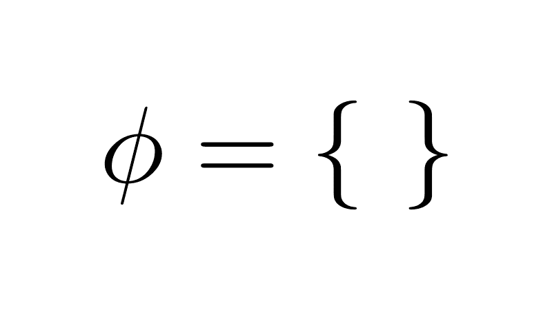
print(s) # {'chair', 'table'}What is a Set?
Order does not matter.
Chronology of Set Operations
- Union (∪) - 1873 - Georg Cantor
- Intersection (∩) - 1873 - Georg Cantor
- Difference (−) - 1873 - Georg Cantor
- Complement (ᶜ) - 1888 - Richard Dedekind
- Logic operators (∨, ∧, ¬) - 1879–1890s - Frege / Peirce

Set Operators and Logical Operators
- Union (∪) ↔ OR (∨)
- Intersection (∩) ↔ AND (∧)
- Complement (ᶜ) ↔ NOT (¬)
- Difference (−) ↔ AND NOT (∧¬)
Sets:
A = {1, 2}
B = {2, 3}

A ∪ B = {1, 2, 3}
A ∩ B = {2}

Logic:
P(x): x ∈ A
Q(x): x ∈ B

P(x) ∨ Q(x): true for 1,2,3
P(x) ∧ Q(x): true for 2
¬P(x): true for 3,4
s = {"chair", "table"}
print(len(s))    # 2

s.add("chair")   # ignored
s.add("desk")    # added
s.add("chair")   # ignored again

print(len(s))    # still 3
print(s) # {'chair', 'table', 'desk'}CREATE TABLE Furniture (
id INTEGER PRIMARY KEY AUTOINCREMENT,
item VARCHAR(50) UNIQUE
);
INSERT INTO Furniture (item) VALUES ('chair'), ('table');
-- Duplicate item → raises exception
INSERT INTO Furniture (item) VALUES ('chair');
-- Error: UNIQUE constraint failed: Furniture.item
-- Using OR IGNORE to mimic set (duplicates ignored)
INSERT OR IGNORE INTO Furniture (item) VALUES ('chair');
INSERT OR IGNORE INTO Furniture (item) VALUES ('desk');
INSERT OR IGNORE INTO Furniture (item) VALUES ('chair');
SELECT COUNT(*) FROM Furniture; -- 3
Set = {chair, table, lamp} with no duplicates
const furniture = new Set([
  "chair",
  "table",
  "lamp"
]);Set<String> furniture = new HashSet<>();
furniture.add("chair");
furniture.add("table");
furniture.add("lamp");furniture = {"chair", "table", "lamp"}CREATE TABLE Furniture (
item INTEGER PRIMARY KEY
);
INSERT INTO Furniture VALUES
('chair'), ('table'), ('lamp');Set Theory: Basic Concept & Use Cases (~1870–1890)
- Set: collection of things
- No duplicates allowed
- Union: combine sets
- Intersection: find common
- Difference: remove one
- Compare set sizes
- Organize & count clearly
- Crop yield forecasting data
- Land parcel boundary mapping
- Soil type classification
- Weather pattern analysis
- Farm census comparisons
- Infinite resource allocation
- Plant breeding statistics
Set Theory – Core Ideas
- Developed by Georg Cantor (late 19th century)
- No duplicates – ensures clarity
- Key operations: union, intersection, difference
- Foundation for relational algebra

Set Operations Summary
| Operation | Symbol | Description | Diagram |
|---|---|---|---|
| Union | ⋃ | All unique elements |  |
| Intersection | ∩ | Common elements only |  |
| Difference | − | In A but not in B |  |
Set Theory Concepts – Visual Overview


What is a Tuple?
Ordered sequence of elements
- (1, 'Trek', 'Mountain', 1200)
- (1, 'Trek', 'Mountain', 1200)
- (1, 'Trek', 'Mountain', 1200)
- (2, 'Giant', 'Road', 1500)
- (3, 'Cannondale', 'Hybrid', 1000)
Bicycles relation:
bikeId | brand      | type     | price
1      | Trek       | Mountain | 1200   ← tuple 1
1      | Trek       | Mountain | 1200   ← tuple 1
1      | Trek       | Mountain | 1200   ← tuple 1
2      | Giant      | Road     | 1500   ← tuple 2
3      | Cannondale | Hybrid   | 1000   ← tuple 3

Each row = one tuple (ordered sequence of elements)Relation = Set of Tuples
- No duplicate rows
- All tuples have the same attributes
- Example schema: Bikes(bikeId, brand, type, price)
Bikes relation (a set of tuples):

bikeId | brand      | type     | price
1      | Trek       | Mountain | 1200
2      | Giant      | Road     | 1500
3      | Cannondale | Hybrid   | 1000

• Each row = one tuple
• No duplicate rows allowed
• All rows share the same columns (attributes)
Relational Algebra Flow
(Set of Tuples)
(Set of Tuples)
Relational Algebra Operators
Selection (σ)
- Filters rows based on condition
- Reduces number of tuples
- Example: σ(price < 1200)(Bicycles)
Input Bicycles:
bikeId | brand      | type     | price
1      | Trek       | Mountain | 1699
2      | Giant      | Road     | 1100
3      | Cannondale | Hybrid   |  999

After σ(price < 1200):
bikeId | brand      | type     | price
2      | Giant      | Road     | 1100
3      | Cannondale | Hybrid   |  999
Projection (π)
- Selects specific columns
- Removes unwanted attributes & duplicates
- Example: π(brand, price)(Bicycles)
Input:
bikeId | brand | model     | price | color
1      | Trek  | Roscoe 7  | 1699  | Blue
2      | Giant | Contend   | 1299  | Black
3      | Trek  | Marlin 5  |  799  | Red

After π(brand, price):
brand | price
Trek  | 1699
Giant | 1299
Trek  |  799
Union (⋃)
- Combines two compatible relations
- Removes duplicates
- Example: Available ⋃ Sold
Available:
bikeId | brand
1      | Trek
2      | Giant

Sold:
bikeId | brand
2      | Giant
4      | Scott

After Union:
bikeId | brand
1      | Trek
2      | Giant
4      | Scott
Set Difference (−)
- Tuples in first but not in second
- Example: Stock − Sold
Stock:
bikeId | brand
1      | Trek
2      | Giant
3      | Cannondale

Sold:
bikeId | brand
2      | Giant

After Difference:
bikeId | brand
1      | Trek
3      | Cannondale
Cartesian Product (×)
- All possible combinations of tuples
- Example: Bikes × Stores
Bikes (2 rows) × Stores (2 rows) = 4 rows

Bikes:     Stores:
1 Trek     A Berlin
2 Giant    B Munich

Result:
bikeId | brand | store | city
1      | Trek  | A     | Berlin
1      | Trek  | B     | Munich
2      | Giant | A     | Berlin
2      | Giant | B     | Munich
Natural Join (⨝)
- Cartesian + equality on shared attribute names
- Example: Orders ⨝ Customers
Orders:                Customers:
orderId | custId | amt    custId | name
101     | 5      | 299    5      | Alice
102     | 7      | 450    7      | Bob

After Natural Join:
orderId | custId | amt | name
101     | 5      | 299 | Alice
102     | 7      | 450 | Bob
Division (÷)
- Tuples in left that match ALL values in right
- Example: Students ÷ RequiredCourses
Enrollments:           Required:
student | course          course
A       | Math            Math
A       | Physics         Physics
B       | Math

After Division (students who took ALL required):
student
A
Renaming (ρ)
- Renames relation or attributes
- Example: ρ(Inv)(Bicycles)
Before:
bikeId | brand | price

After ρ(Inv ← Bicycles):
Inv.bikeId | Inv.brand | Inv.price
Relational Algebra Operators – Summary
| Operator | Symbol | Description | Example |
|---|---|---|---|
| Selection | σ | Filter rows | σ(price < 1200)(Bikes) |
| Projection | π | Select columns | π(brand, price)(Bikes) |
| Union | ⋃ | Combine, no duplicates | Avail ⋃ Sold |
| Difference | − | A minus B | Stock − Sold |
| Cartesian Product | × | All pairs | Bikes × Stores |
| Natural Join | ⨝ | Match on common attrs | Orders ⨝ Customers |
| Division | ÷ | Match all values | Students ÷ Required |
| Renaming | ρ | Rename relation/attrs | ρ(Inv)(Bikes) |
Query Optimization
Optimization Principles
- Reduce rows early
- Reduce columns early
- Delay large joins
σ  → less rows
π  → less columns
⨝  → less comparisons
Execution Flow
- Logical order of operations
- Goal is small intermediates
Relations
   ↓
Selection
   ↓
Projection
   ↓
Join
   ↓
Result
Pushing Selection Down
- Apply filters before joins
- Joins touch less tuples
Before:
π brand (σ price < 500 (Bicycles ⨝ Stores))

After:
π brand ((σ price < 500 (Bicycles)) ⨝ Stores)
Pushing Selection Down
Slow (filter late)
Step 1: Bicycles ⨝ Stores
  → large intermediate result

Step 2: σ price < 500
  → many rows discarded late

π brand
Fast (filter early)
Step 1: σ price < 500 (Bicycles)
  → small input

Step 2: filtered Bicycles ⨝ Stores
  → fewer comparisons

π brand
Combining Projections
- Nested projections collapse
- Remove unused columns once
Before:
π brand (π bikeId, brand (Bicycles))

After:
π brand (Bicycles)
Eliminating Unnecessary Joins
- No attributes used from table
- No predicates applied
Before:
π brand (Bicycles ⨝ Stores ⨝ Suppliers)

After:
π brand (Bicycles ⨝ Stores)
Reordering Joins
- Associative
- Commutative
- Cost changes, result does not
(Bicycles ⨝ Stores) ⨝ Suppliers

Bicycles ⨝ (Stores ⨝ Suppliers)
Join Reordering
- Orders (O): 1,000,000
- Customers (C): 100,000
- Regions (R): 10
Query:
σ R.name = 'West' (O ⨝ C ⨝ R)
Join Reordering – Bad Order
- Large intermediate result
- Filtering happens late
(O ⨝ C) ⨝ R

O ⨝ C → ~100,000,000,000 rows
Join Reordering – Better Order
- Filter small relation first
- Join reduced inputs
O ⨝ (C ⨝ (σ R='West'(R)))

R: 10 → 1
C: 100,000 → 10,000
O ⨝ C → ~1,000,000,000 rows
Selection and Projection Pushdown
- less rows
- less columns
Before:
σ price < 500 (π brand, price (Bicycles ⨝ Stores))

After:
(π brand, price (σ price < 500 (Bicycles)))
⨝ Stores
Example Query
- Flowers over $10
- Only roses
- Local suppliers
σ Price > 10 ∧ Name='Rose' ∧ Location='Local'
(Flowers ⨝ Suppliers)
Without Optimization
- Join first
- Filter later
Flowers ⨝ Suppliers
→ apply filters

1,000 × 500 = 500K
With Optimization
- Filter first
- Join reduced sets
(σ Local (Suppliers))
⨝
(σ Rose ∧ Price > 10 (Flowers))

100 × 50 = 5K
Large Join Graph
- Flowers: 1,000,000
- Suppliers: 200,000
- Supply: 5,000,000
(σ Rose ∧ Red (Flowers))
⨝ Supply
⨝ (σ Local (Suppliers))
Nested Relational Algebra
- Deeply nested joins
- Multiple selections
π Name (
  σ Price > 10 (
    Flowers ⨝
    (σ Local (Suppliers ⨝
      σ Revenue > 1000 (Companies)))
  )
)
Optimized Nested Form
- Selections pushed down
- Smaller joins
π Name (
  (σ Price > 10 (Flowers))
  ⨝
  (σ Local (Suppliers ⨝
     σ Revenue > 1000 (Companies)))
)
Relational Algebra vs SQL
- Logical rules
- Query equivalence
- Executable language
- Cost based optimizer
Practice Questions
- Which join order produces the smallest intermediate result?
- Where should selections be applied?
- Which projections can be pushed down?
- Why does join order affect performance?
SQLite Timing and Setup
- .timer on shows execution time
- journal_mode OFF avoids disk logging
- synchronous OFF skips fsync
- temp_store MEMORY keeps temp data in RAM
- Used only for benchmarking
- Makes slow vs fast visible
- Not for production use
journal_mode = OFF
- Disables rollback journal
- No crash recovery
- Fast writes
Write Operation
     ↓
[ No Journal ]
     ↓
Data File
synchronous = OFF
- Skips fsync
- OS buffers writes
- Lower latency
SQLite
  ↓ write
OS Buffer
  ↓ (later)
Disk
temp_store = MEMORY
- Temporary tables
- Intermediate results
- No temp disk files
Query
  ↓
Temp Tables
  ↓
RAM (Memory)
ANALYZE
- Collects table statistics
- Estimates row counts
- Improves join order
- Helps cost-based optimizer
- No data modification
- Run after bulk inserts
Data Generation (Concept)
- Generate sequences internally
- No external files
- Large but controlled datasets
- Skewed values create selectivity
- Few matches, many non-matches
- Highlights optimization impact
Data Generation (Concept)
- Internal sequence generation
- No external data files
- Deterministic and repeatable
Sequence (1…N)
      ↓
Value assignment
      ↓
Skew introduced
      ↓
Large tables
Set-Based INSERT (Concept)
- Single SQL statement
- Many rows inserted
- No application loop
- Set based execution
seq = [1, 2, 3, ..., 200000]
INSERT customers
FOR EACH x IN seq:
  (x, 'West' or 'Other')
Data Generation (SQL Structure)
- Recursive query generates numbers
- COUNT defines table size
- Abort condition stops recursion
WITH RECURSIVE
  seq(x)
      ↓
x starts at 1
      ↓
x = x + 1
      ↓
STOP when x reaches limit
      ↓
INSERT generated rows
Recursive Data Generation
-- Define a recursive sequence
WITH RECURSIVE seq(x) AS (
  -- Base case: start at 1
  SELECT 1

  UNION ALL

  -- Recursive step: increment
  SELECT x + 1
  FROM seq

  -- Abort condition
  WHERE x < 200000
)
-- Insert generated values
INSERT INTO customers
SELECT
  x,                     -- unique id
  CASE                   -- controlled skew
    WHEN x % 100 = 0
    THEN 'West'
    ELSE 'Other'
  END
FROM seq;
What is x in seq(x)?
xis the column name of the recursive tableseqis a temporary result set- Each row in
seqhas one value:x seq= table,x= column
WITH RECURSIVE seq(x) AS (...)

seq
----
x
----
1
2
3
...
Wall Clock Time vs CPU Time
- Wall clock = total elapsed time
- User = CPU executing query
- Sys = OS and kernel work
Time ─────────────────────────────▶

|──────────── real (wall clock) ────────────|

|──────── user (CPU work) ───────|

| sys |


Example:
real = user + sys + waiting
      (what the user feels)
Understanding SQLite Timing Output
- real: wall-clock time
- user: CPU time in SQLite
- sys: OS-level overhead
Run Time:
real 0.077
user 0.075025
sys  0.000000
- ~77 ms total execution
- Mostly CPU work
- Negligible system cost
SQLite Demo
- Same query result
- Different execution time
Practice 1
SELECT COUNT(*)
FROM orders o
JOIN customers c ON o.customer_id = c.customer_id
WHERE c.region = 'West';
- How would you make this faster?
- Which table should be filtered first?
σ region='West' (Orders ⨝ Customers)
Practice 2
SELECT *
FROM sales s
JOIN products p ON s.product_id = p.id
WHERE p.category = 'Bike';
- Where should selection be applied?
σ category='Bike' (Sales ⨝ Products)
Practice 3
SELECT o.id
FROM orders o
JOIN customers c ON o.customer_id = c.customer_id
JOIN regions r ON c.region_id = r.id
WHERE r.name = 'West';
- Which join should happen first?
Orders ⨝ (Customers ⨝ σ name='West' (Regions))
Practice 4
SELECT *
FROM enrollments e
JOIN students s ON e.student_id = s.id
WHERE s.major = 'CS';
- How to reduce intermediate size?
Enrollments ⨝ σ major='CS' (Students)
Practice 5
SELECT *
FROM supply sp
JOIN suppliers s ON sp.supplier_id = s.id
JOIN flowers f ON sp.flower_id = f.id
WHERE s.location = 'Local';
- Which table is most selective?
Supply ⨝ (σ location='Local' (Suppliers) ⨝ Flowers)
Practice 6
SELECT *
FROM logs l
JOIN users u ON l.user_id = u.id
WHERE u.active = 1;
- Which relation should be reduced first?
Logs ⨝ σ active=1 (Users)
Practice 7
SELECT *
FROM orders o
JOIN items i ON o.id = i.order_id
WHERE o.date > '2025-01-01';
- What happens if we filter orders first?
σ date>'2025-01-01' (Orders) ⨝ Items
Practice 8
SELECT *
FROM activity a
JOIN conditions c ON a.id = c.activity_id
WHERE c.type = 'once';
- Where is the selective predicate?
Activity ⨝ σ type='once' (Conditions)
Practice 9
SELECT *
FROM payments p
JOIN users u ON p.user_id = u.id
JOIN countries c ON u.country_id = c.id
WHERE c.code = 'US';
- Which join should be last?
Payments ⨝ (Users ⨝ σ code='US' (Countries))
Practice 10
SELECT *
FROM reviews r
JOIN products p ON r.product_id = p.id
WHERE p.rating > 4;
- How does early filtering help?
Reviews ⨝ σ rating>4 (Products)
Answer 1
SELECT COUNT(*)
FROM (
  SELECT customer_id
  FROM customers
  WHERE region = 'West'
) c
JOIN orders o ON o.customer_id = c.customer_id;
-- Before
σ region='West' (Orders ⨝ Customers)

-- After
Orders ⨝ (π customer_id (σ region='West' (Customers)))
Answer 2
SELECT s.sale_id, s.product_id, s.qty
FROM (
  SELECT id
  FROM products
  WHERE category = 'Bike'
) p
JOIN sales s ON s.product_id = p.id;
-- Before
σ category='Bike' (Sales ⨝ Products)

-- After
Sales ⨝ (π id (σ category='Bike' (Products)))
Answer 3
SELECT o.id
FROM (
  SELECT id
  FROM regions
  WHERE name = 'West'
) r
JOIN customers c ON c.region_id = r.id
JOIN orders o ON o.customer_id = c.customer_id;
-- Before
π o.id (σ name='West' (Orders ⨝ Customers ⨝ Regions))

-- After
π o.id (
  Orders ⨝
  (Customers ⨝ (π id (σ name='West' (Regions))))
)
Answer 4
SELECT e.student_id, e.course_id
FROM enrollments e
JOIN (
  SELECT id
  FROM students
  WHERE major = 'CS'
) s ON e.student_id = s.id;
-- Before
σ major='CS' (Enrollments ⨝ Students)

-- After
Enrollments ⨝ (π id (σ major='CS' (Students)))
Answer 5
SELECT sp.supplier_id, sp.flower_id
FROM (
  SELECT id
  FROM suppliers
  WHERE location = 'Local'
) s
JOIN supply sp ON sp.supplier_id = s.id
JOIN flowers f ON sp.flower_id = f.id;
-- Before
σ location='Local' (Supply ⨝ Suppliers ⨝ Flowers)

-- After
((Supply ⨝ (π id (σ location='Local' (Suppliers)))) ⨝ Flowers)
Answer 6
SELECT l.log_id, l.user_id, l.action
FROM logs l
JOIN (
  SELECT id
  FROM users
  WHERE active = 1
) u ON l.user_id = u.id;
-- Before
σ active=1 (Logs ⨝ Users)

-- After
Logs ⨝ (π id (σ active=1 (Users)))
Answer 7
SELECT o.id, i.item_id, i.qty
FROM (
  SELECT id
  FROM orders
  WHERE date > '2025-01-01'
) o
JOIN items i ON o.id = i.order_id;
-- Before
σ date>'2025-01-01' (Orders ⨝ Items)

-- After
((π id (σ date>'2025-01-01' (Orders))) ⨝ Items)
Answer 8
SELECT a.id, a.title, c.type
FROM activity a
JOIN (
  SELECT activity_id, type
  FROM conditions
  WHERE type = 'once'
) c ON a.id = c.activity_id;
-- Before
σ type='once' (Activity ⨝ Conditions)

-- After
Activity ⨝ (π activity_id, type (σ type='once' (Conditions)))
Answer 9
SELECT p.payment_id, p.amount
FROM (
  SELECT id
  FROM countries
  WHERE code = 'US'
) c
JOIN users u ON u.country_id = c.id
JOIN payments p ON p.user_id = u.id;
-- Before
π payment_id, amount (σ code='US' (Payments ⨝ Users ⨝ Countries))

-- After
π payment_id, amount (
  Payments ⨝
  (Users ⨝ (π id (σ code='US' (Countries))))
)
Answer 10
SELECT r.review_id, r.product_id, r.stars
FROM reviews r
JOIN (
  SELECT id
  FROM products
  WHERE rating > 4
) p ON r.product_id = p.id;
-- Before
σ rating>4 (Reviews ⨝ Products)

-- After
Reviews ⨝ (π id (σ rating>4 (Products)))
Module 4
Relational Database Interfaces
                 ┌──────────────────────┐
                 │   Admin Interface    │
                 │  (CLI · GUI · Tools) │
                 └──────────┬───────────┘
                            │
                            │
┌──────────────────────┐    │    ┌──────────────────────┐
│  Application Code    │────┼────│   Data Tools / ETL   │
│ (Web · Mobile · API) │    │    │  (Import · Export)   │
└──────────┬───────────┘    │    └──────────┬───────────┘
           │                │               │
           │                ▼               │
           │        ┌────────────────┐      │
           └───────▶      DBMS       ◀─────┘
                    │ (SQLite / PG)  │
                    │  parse · exec  │
                    │  enforce rules │
                    └────────────────┘
                            ▲
                            │
                 ┌──────────┴───────────┐
                 │   Reporting / BI     │
                 │  (Queries · Views)   │
                 └──────────────────────┘
Today
- Practice Questions
- Relational Database Interfaces:
- Admin Interface
- Command-Line Interface (CLI)
- Application Programming Interface (API)
- Application User Interface (UI)
- PostgreSQL
- Homework 2, Lab 2

1970s: The Relational Model Becomes Real
- Relational model introduced
- Research prototypes
- Early query languages
- Interfaces are terminals

Early Client–Database: Terminal Direct (Before GUI)
- Users worked directly in a terminal
- No graphical tools: only text commands and scripts
- SQL typed manually and executed immediately
- Automation came from shell scripts and batch jobs
- Fast and precise, but less friendly for non technical users
┌──────────────────────┐
│        User          │
│ (DBA · Developer)    │
└──────────┬───────────┘
           │
           ▼
┌──────────────────────┐
│      Terminal        │
│ (CLI · Shell)        │
│ SQL · scripts        │
└──────────┬───────────┘
           │
           │ SQL / Batch Jobs
           ▼
┌──────────────────────┐
│       Database       │
│ (Tables · Rules)     │
│ constraints · ids    │
└──────────────────────┘
1980s: Commercial RDBMS and Admin Tools
- Relational databases enter mainstream
- DBA role becomes formal
- Vendor tooling grows
- GUIs appear
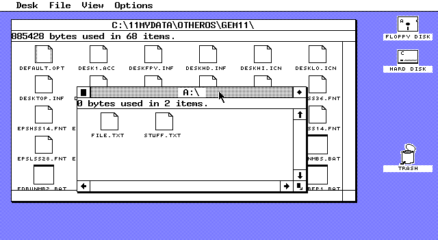
Client–Database Architecture with GUI in Between
- Users do not talk to the database directly
- A GUI sits between the user and the database
- The GUI translates user actions into queries
- The database remains protected and structured
- This pattern scales from desktop apps to the web
┌──────────────────────┐
│        User          │
│ (Clicks · Forms)     │
└──────────┬───────────┘
           │
           ▼
┌──────────────────────┐
│        GUI           │
│ (Desktop · Web UI)   │
│ buttons · tables     │
└──────────┬───────────┘
           │
           │ SQL / Queries
           ▼
┌──────────────────────┐
│       Database       │
│ (Tables · Rules)     │
│  constraints · ids   │
└──────────────────────┘
1990s: SQL Standardization and CLI Automation
- SQL becomes the common language across systems
- Scripting and batch jobs become normal operations
- ODBC and JDBC spread database connectivity
- Client tools focus on productivity forDBAs
2000s: APIs Everywhere and 3 Tier Applications
- Apps standardize frontend, backend, database tiers
- Drivers mature across languages (eg. Java)
- Connection pooling and app servers
- Security push access through backend services
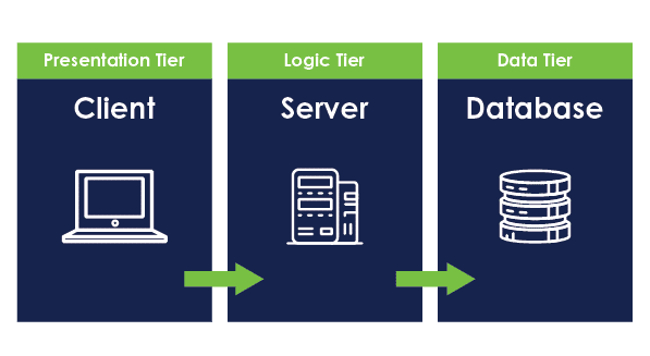
Three Tier Architecture with Internet
- Users access the system over the internet
- Frontend handles presentation and user interaction
- Backend enforces business logic and security
- Database is never exposed directly to users
- This becomes the dominant web architecture
┌──────────────────────┐
│        User          │
│ (Browser · Client)   │
└──────────┬───────────┘
           │ Internet (HTTP / HTTPS)
           ▼
┌──────────────────────┐
│      Frontend        │
│ (Web UI · Forms)     │
│ HTML · CSS · JS      │
└──────────┬───────────┘
           │ API Calls
           ▼
┌──────────────────────┐
│       Backend        │
│ (Logic · Auth)       │
│ REST · Validation    │
└──────────┬───────────┘
           │ SQL
           ▼
┌──────────────────────┐
│       Database       │
│ (Tables · Rules)     │
│ constraints · ids    │
└──────────────────────┘
2010s: Web Consoles, Cloud, and Self Service Data
- Managed database web based admin consoles
- Infrastructure automation becomes routine
- BI dashboards spread to non technical users
- Identity, roles, auditing, and encryption

Cloud Native Architecture (Logical View)
- Workloads are split into independent cloud services
- Frontend and backend scale separately
- Databases run as managed cloud services
- Infrastructure concerns are abstracted away
- Everything communicates over secure networks
┌──────────────────────┐      ┌──────────────────────┐
│        Users         │      │     Cloud Platform   │
│ (Browser · Mobile)   │      │ (Network · Policy)   │
└──────────┬───────────┘      └──────────┬───────────┘
           │                               │
           │ Internet (HTTPS)              │ Managed Services
           ▼                               ▼
┌──────────────────────┐      ┌──────────────────────┐
│ Cloud App Services   │      │  Cloud Database      │
│ (Frontend + Backend) │      │ (Managed RDBMS)      │
│ APIs · Auth · Logic  │      │ backups · replicas   │
└──────────────────────┘      └──────────────────────┘
2020+: Hybrid Interfaces and Assisted Operations
- Hybrid workflows: CLI + web UI + APIs
- Policy driven security and compliance
- Observability becomes first class
- Automation and assistants
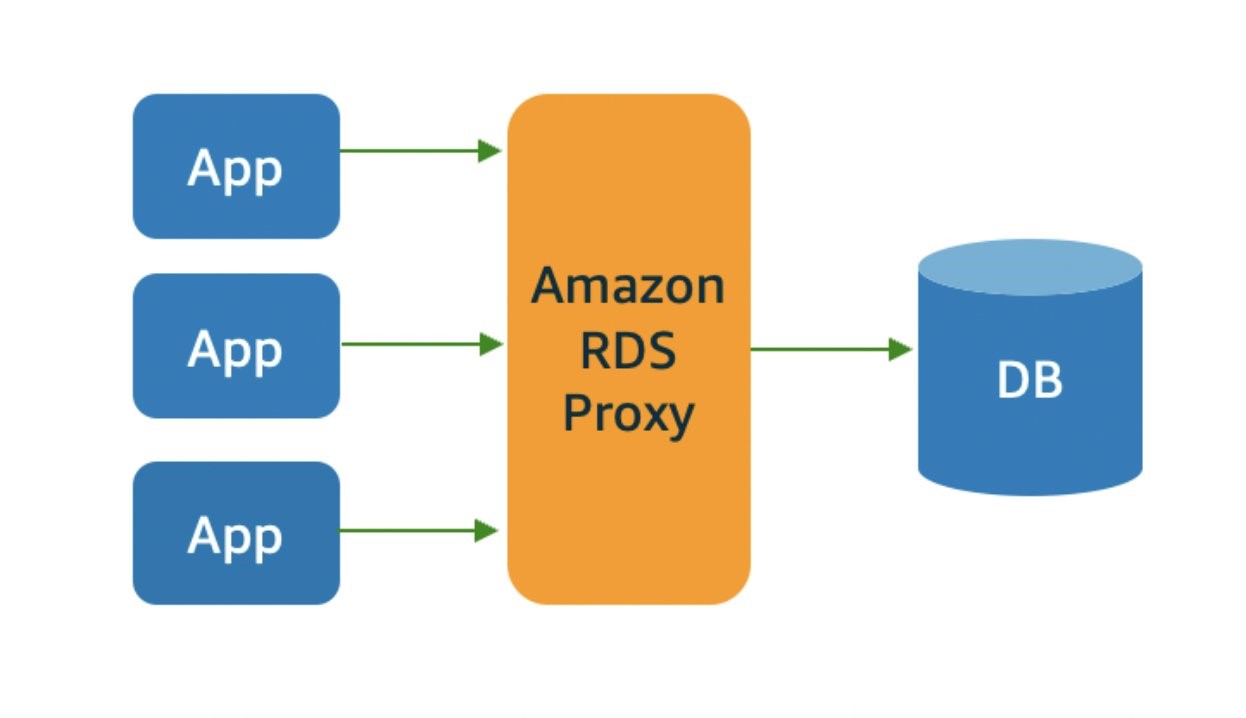
What is a relation?
- A collection of duplicate tuples
- A single row in a table
- A function mapping keys to values
- A set of unique tuples with the same attributes
Which SQL clause is used to filter rows before processing?
- WHERE
- HAVING
- GROUP BY
- ORDER BY
Which relational algebra operation eliminates duplicate tuples?
- Selection (σ)
- Projection (π)
- Union (∪)
- Difference (-)
Which SQL statement correctly defines a foreign key constraint?
CREATE TABLE Orders (OrderID INT PRIMARY KEY, CustomerID INT FOREIGN KEY REFERENCES Customers(CustomerID)); -- A

CREATE TABLE Orders (OrderID INT, CustomerID INT, FOREIGN KEY (CustomerID) REFERENCES Customers(CustomerID)); -- B

CREATE TABLE Orders (OrderID INT, CustomerID INT, FOREIGN KEY REFERENCES Customers(CustomerID)); -- C

CREATE TABLE Orders (OrderID INT PRIMARY KEY, FOREIGN KEY (CustomerID) REFERENCES Customers(CustomerID)) -- D
Which SQL query is optimized?
- σage > 30 (Users ⨝ Orders)
- (σage > 30 Users) ⨝ Orders
- σage > 30 ((Users ⨝ Orders))
- (Users ⨝ Orders) ⨝ σage > 30 (Users)
Which SQL statement is correct?
CREATE TABLE Table (ID INT PRIMARY KEY, Name VARCHAR(50));

CREATE TABLE Orders (OrderID INT, CustomerID INT, FOREIGN KEY (CustomerID) REFERENCES Customers(CustomerID))

CREATE TABLE Orders (OrderID INT, CustomerID INT, FOREIGN KEY REFERENCES Customers(CustomerID));

CREATE TABLE Orders (OrderID INT, FOREIGN KEY (CustomerID) REFERENCES Customers(CustomerID), CustomerID INT);

CREATE TABLE Orders (OrderID INT, CustomerID INT, FOREIGN KEY (CustomerID) REFERENCES Customers(CustomerID));
What is the relationship between Customers and Orders, where one customer can have multiple orders?
- One-to-One (1:1)
- One-to-Many (1:N)
- Many-to-Many (N:N)
- One-to-Many (N:1)
Which relational algebra operator is used to retrieve specific attributes?
- Projection (π)
- Selection (σ)
- Cartesian Product (×)
- Union (∪)
In query optimization, which heuristic helps reduce the number of tuples early?
- Predicate Pushdown
- Join Reordering
- Expression Flattening
- Index Lookup
Relational Database Interfaces
- Databases are stable
- Interfaces change often
- Each interface fits a role
                 ┌──────────────────────┐
                 │   Admin Interface    │
                 │  (CLI · GUI · Tools) │
                 └──────────┬───────────┘
                            │
                            │
┌──────────────────────┐    │    ┌──────────────────────┐
│  Application Code    │────┼────│   Data Tools / ETL   │
│ (Web · Mobile · API) │    │    │  (Import · Export)   │
└──────────┬───────────┘    │    └──────────┬───────────┘
           │                │               │
           │                ▼               │
           │        ┌────────────────┐      │
           └───────▶      DBMS       ◀─────┘
                    │ (SQLite / PG)  │
                    │  parse · exec  │
                    │  enforce rules │
                    └────────────────┘
                            ▲
                            │
                 ┌──────────┴───────────┐
                 │   Reporting / BI     │
                 │  (Queries · Views)   │
                 └──────────────────────┘
Evolution of Relational Database Interfaces
- 1970s: Early Databases
- 1980s: Admin Tools Emerge
- 1990s: Command-Line Interface (CLI)
- 2000s: APIs Enable Integration
- 2010s: Web-Based Interfaces
- Today: Hybrid and Automated Systems
Time
  ↓
GUI tools
  ↓
CLI automation
  ↓
APIs for apps
  ↓
Web dashboards
Database Interfaces by Role and Purpose
| Interface | Role | Purpose | Technology |
|---|---|---|---|
| Admin Interface (GUI) | Database Administrators | User management, schema modifications, monitoring | SQLite Browser |
| Command-Line Interface (CLI) | Developers and DBAs | Direct SQL execution, automation, scripting | SQLite CLI |
| Application Programming Interface (API) | Developers | Programmatic database interaction, integrating apps | Neon Tech |
| Web-Based UI | Regular Users | Accessing, viewing, and interacting with data in a user friendly way | - |
What is a Direct Database API Interface?
- Application connects to the database directly
- Uses a driver and connection string
- Runs SQL without HTTP
App
  ↓ (driver)
Database
  ↓
SQL results
Direct Database API
- Connects online directly to a database using drivers
Driver examples:
psycopg2 (Python)
pg (Node)
JDBC (Java)
Database Connection
- Uses a connection string
- Contains host, database, user, SSL mode
postgresql://user:password@host:port/database?sslmode=requireDirect DB API vs REST API
- Direct DB API: Uses drivers for queries
- Lower overhead, higher exposure
- REST API: Uses HTTP endpoints
- Backend controls access and validation
Security
- Use authentication (user/pwd, certificates)
- Restrict access with roles and permissions
- Enable SSL and TLS for encryption
Risk increases when DB is exposed
Prefer:
App → Backend → DB
over:
App → DB
Python Connection
- Driver: psycopg2
- Connection string
- Simple query
import psycopg2
conn = psycopg2.connect("postgresql://user:pass@host/db?sslmode=require")
cur = conn.cursor()
cur.execute("SELECT version();")
print(cur.fetchone())
Best Practices
- Use connection pooling
- Restrict database exposure
- Sanitize inputs to prevent SQL injection
Keep credentials out of code
Least privilege roles
Rotate secrets
Furniture Application: System Tiers
Frontend
User interface
Forms · Buttons · Lists
Backend
Application logic
Validation · APIs
Database
Data storage
Tables · Constraints
Checkout Database Repository
- Clone the repository
- Navigate to the project directory
git clone https://github.com/SE4CPS/2026-COMP-163cd 2026-COMP-163Database Interfaces by Role and Purpose
| Interface | Role | Purpose | Technology |
|---|---|---|---|
| Admin Interface (GUI) | Database Administrators | User management, schema modifications, monitoring | SQLite Browser |
| Command-Line Interface (CLI) | Developers and DBAs | Direct SQL execution, automation, scripting | SQLite CLI |
| Application Programming Interface (API) | Developers | Programmatic database interaction, integrating apps | Neon Tech |
| Web-Based UI | Regular Users | Accessing, viewing, and interacting with data in a user friendly way | - |
What is a Admin Tool Interface?
Today
- Relational Database Admin Interfaces
- Introduction PostgreSQL
- Relational Database Developer Interfaces
- Relational Database User Interfaces
- Practice Questions
Admin  → database ownership tasks
Dev    → build apps on top
User   → consume data safely
Admin Interface
Database Ownership Tasks
CLI · GUI · Tools
backups · users · schema · monitoring
┌──────────────────────┐
│ Admin Interface │
│ (CLI · GUI · Tools) │
└──────────┬───────────┘
│
│
┌──────────────────────┐ │ ┌──────────────────────┐
│ Application Code │────┼────│ Data Tools / ETL │
│ (Web · Mobile · API) │ │ │ (Import · Export) │
└──────────┬───────────┘ │ └──────────┬───────────┘
│ │ │
│ ▼ │
│ ┌────────────────┐ │
└───────▶ DBMS ◀─────┘
│ (SQLite / PG) │
│ parse · exec │
│ enforce rules │
└────────────────┘
▲
│
┌──────────┴───────────┐
│ Reporting / BI │
│ (Queries · Views) │
└──────────────────────┘
What is an Admin Interface?
- It is the control surface for a database system
- Used by DBAs, platform engineers, and senior devs
- Focus: ownership tasks, safety, repeatability, audit
- Includes roles, backups, perf, schema changes
Traditional rule: treat admin actions like production change control.
Admin Interface = "How we control the DB"
Not:
- how users browse data
- how apps call SQL
Yes:
- how owners keep it stable
Admin Interface Task Map
| Area | Typical Tasks | Why it matters | Common Tools |
|---|---|---|---|
| Identity | Users, roles, grants, password rotation | Least privilege | psql, pgAdmin, cloud console |
| Reliability | Backups, restore tests, replication checks | Recovery time | pg_dump, snapshots |
| Schema | Migrations, constraints, indexes, data fixes | Correctness | migration tools, SQL |
| Observability | Slow queries, locks, storage growth, alerts | Predictability | metrics, logs, dashboards |
CLI vs GUI for Admin Work
CLI (traditional)
- Scriptable and repeatable
- Easy to review in change logs
- Works over slow links
- Good for emergency response
psql
pg_dump / pg_restore
SQL scripts
cron / CI jobs
GUI (operational)
- Discoverability: browse schema and settings
- Good for onboarding and spot checks
- Lower barrier for safe read only work
- Must be used carefully for write actions
pgAdmin
DBeaver
SQLite Browser
Cloud consoles
Admin Controls Access: Roles and Grants
- Admin defines roles first
- Roles get permissions (not individual users)
- Apps run with service accounts
- Auditing requires predictable role design
┌──────────────┐ grants ┌──────────────┐
│ Admin │──────────────────▶│ Role │
│ (owner) │ │ (policy) │
└──────┬───────┘ └──────┬───────┘
│ │
│ assigns │ used by
▼ ▼
┌──────────────┐ ┌──────────────┐
│ User │ │ App │
│ (human) │ │ (service) │
└──────┬───────┘ └──────┬───────┘
│ │
└────────────── SQL ───────────────┘
▼
┌──────────────┐
│ DBMS │
│ checks rules │
└──────────────┘
Backups: The Most Important Admin Habit
- Backups are only real if restore is tested
- Prefer scheduled, automated backups
- Keep copies separated from the primary system
- Track: RPO (data loss) and RTO (recovery time)
Traditional rule: practice restore like a fire drill.
┌──────────────┐ pg_dump ┌──────────────┐
│ Primary │─────────────────▶│ Backup │
│ DBMS │ │ Store │
└──────┬───────┘ └──────┬───────┘
│ │
│ restore test │ retention
▼ ▼
┌──────────────┐ pg_restore ┌──────────────┐
│ Staging DB │◀────────────────│ Policies │
│ (verification) │ (30d / 90d) │
└──────┬───────┘ └──────────────┘
│
▼
confidence report
Schema Changes: Safe Admin Workflow
- Schema is a contract between apps and data
- Changes should follow a predictable sequence
- Prefer migration scripts under version control
| Step | Action | Admin goal |
|---|---|---|
| 1 | Plan change | Know impact |
| 2 | Run in staging | Catch issues early |
| 3 | Deploy during window | Minimize disruption |
| 4 | Validate with queries | Confirm correctness |
| 5 | Record + audit | Traceability |
Monitoring: What Admins Watch
- Slow queries and query volume
- Locks and long transactions
- Disk growth and bloat
- Connection counts and errors
- Replication lag (if used)
Signals → Actions
Slow queries → optimize SQL / add index
Locks → fix transactions
Disk growth → retention / cleanup
Auth failures → rotate secrets / investigate
Backup failures → stop and repair immediately
Where Admin Interface Fits in 3 Tier Architecture
- Users should not reach the database directly
- Apps should access data through a backend
- Admins may access DBMS directly, with strict controls
- Admin access should be logged and limited
┌──────────────────────┐
│ Users │
└──────────┬───────────┘
│ HTTPS
▼
┌──────────────────────┐
│ Frontend │
└──────────┬───────────┘
│ REST
▼
┌──────────────────────┐
│ Backend │
└──────────┬───────────┘
│ SQL
▼
┌──────────────────────┐
│ DBMS │
└──────────┬───────────┘
▲
│ privileged (admin)
┌──────────┴───────────┐
│ Admin Interface │
│ (CLI · GUI · Tools) │
└──────────────────────┘
Quick Check: Is this an Admin Task?
| Task | Admin? | Why |
|---|---|---|
| Creating a backup | Yes | Reliability ownership |
| Managing user permissions | Yes | Policy and access control |
| Writing a new API endpoint | No | Application layer work |
| Building a dashboard view | No | User or BI interface work |
Admin work:
- keeps system stable
- changes ownership settings
- restores service when broken
If it changes policy, backups, or schema:
it is admin.
Admin Interface: Neon for PostgreSQL
- Admin UI for hosted PostgreSQL
- Useful for quick setup and inspection
Admin Interface: DB Browser for SQLite
- Admin GUI for local SQLite databases
- Open .db files and inspect tables
- Run SQL queries and export results (CSV)
- You can see schema and data side by side
Download DB Browser for SQLite
┌──────────────┐ open .db ┌──────────────────────┐
│ Student │ ──────────────▶ │ DB Browser (GUI) │
│ (local file) │ │ tables · schema · SQL│
└──────────────┘ └──────────┬───────────┘
│
▼
┌──────────────┐
│ SQLite DB │
│ tables · rows│
└──────────────┘
Task 1: Creating a Database Backup
Is this an Admin Task, Developer Task, or User Task?
Task 2: Writing a New API Endpoint
Is this an Admin Task, Developer Task, or User Task?
Task 3: Managing User Permissions
Is this an Admin Task, Developer Task, or User Task?
Task 4: Debugging an Application Error
Is this an Admin Task, Developer Task, or User Task?
Task 5: Updating Software Dependencies
Is this an Admin Task, Developer Task, or User Task?
PostgreSQL Queries
- SQLite is useful for learning and local work
- PostgreSQL is used for multi user, production systems
- PostgreSQL specific query behavior
Traditional flow: learn SQLite first, then move to PostgreSQL.
Jump to PostgreSQL section
Relational Database Developer Interfaces
Developers: The Bridge
- Connect frontend applications to databases
- Handle business logic and data processing
- Develop APIs for frontend communication
- Ensure data security and integrity
- Optimize performance between UI and storage
Backend to Database Connection
- Uses API key for authentication
- Connects to PostgreSQL database
- Ensures secure communication with SSL
Backend
↓ (SSL)
PostgreSQL
PostgreSQL API Connection String Breakdown
- Protocol: postgresql://
- Username: neondb_owner
- Password: *********
- Host: ep-shrill-tree-a819xf7v-pooler.eastus2.azure.neon.tech
- Database: neondb
- SSL Mode: require (ensures secure connection)
Backend to Frontend via REST API
- Exposes endpoints for frontend access
- Uses HTTP methods (GET, POST, etc.)
- Requires authentication for secure access
Frontend
↓ HTTP
Backend (REST)
↓ SQL
Database
REST API Request Example
@app.route('/flowers')
def manage_flowers():
conn = get_db_connection()
cur = conn.cursor()
cur.execute("SELECT * FROM flowers")
flowers = cur.fetchall()
cur.close()
conn.close()
return render_template('flowers.html', flowers=flowers)
Task 1: Designing a Database Schema
Is this a Backend Database Developer Task?
Task 2: Implementing a REST API
Is this a Backend Database Developer Task?
Task 3: Styling a Web Page
Is this a Backend Database Developer Task?
PostgreSQL Backend Code Example
GitHub: PostgreSQLQuestions?
Relational Database User Interfaces
Frontend Database Related Tasks
- Fetching data from APIs
- Displaying database records in UI
- Sending user input to backend
- Handling API authentication (e.g., tokens)
- Managing client side caching
- Managing client side validation
PostgreSQL Backend Code Example
GitHub: PostgreSQLQuestion 1
Is fetching data from an API a frontend or backend task?
Question 2
Who is responsible for validating user input before storing it in the database?
Question 3
Does the frontend directly modify the database?
Questions?
Today: Flower Store
- System overview: Flower store
- Interfaces and responsibilities
- Local DB (SQLite) vs Remote DB (Postgres)
- Team project setup
- Role based implementation
- Admin – schema, seed, system setup
- Dev (Backend) – SQL + data access
- Dev (FrontEnd) – Flask routes + UI
- User – inventory and edits
- Customer – communicate requirements
ERD Design – Flower Store
ERD goals
We want to keep track of the flower inventory.
- Identify the main entity
- Choose a primary key
- Select essential attributes
Start on paper before using any tool.
PlantUML template
@startuml
entity FlowerEntity {
* id : int
--
attribute_one : text
attribute_two : text
attribute_three : number
}
@enduml
Design Decision – Which Constraints?
- What must be unique?
- What must be not null?
- What should have a default value?
Constraints protect the data, not the code.
- Can two rows share the same value?
- Can this field ever be empty?
- What value makes sense if none is provided?
Decide at the database level first.
Design Decision – Which Database?
SQLite
- Local database file
- No server process
- Easy to set up
- Good for learning and prototyping
PostgreSQL
- Client–server database
- Runs as a separate service
- Supports concurrent users
- Closer to production systems
Implementation
Starter code
# first time only
git clone https://github.com/SE4CPS/2026-COMP-163.git
# every class / work session
cd 2026-COMP-163
git pull
Why this matters
- Everyone starts from the same baseline
- Updates arrive incrementally
- Interfaces stay consistent
Team Roles – Flower Store
Admin
- Database schema
- Seed data
- System setup
Dev (Backend)
- SQL queries
- CRUD functions
- Database interface
Dev (FrontEnd)
- Flask routes
- Forms and views
- User interactions
User
- Add flowers
- Edit inventory
- Delete entries
Customer
- View inventory
- No edits
- Read only access
Who Handles the Server?
Admin
- Server setup
- Environment configuration
- Database service running
Dev (Backend)
- Application server code
- Flask app logic
- Database connections
Server (Conceptual Role)
- Runs continuously
- Hosts the application
- Exposes endpoints
Key idea
- No UI
- No buttons
- Pure infrastructure
Database Interface and ID
Frontend
Backend
Database
Which component is responsible for ensuring data validation and access control?
- Frontend
- Backend
- Database
- All of the above
Which component plays a key role in optimizing system performance and preventing security breaches?
- Frontend
- Backend
- Database
- All of the above
Which component is essential for managing user requests, processing data, and ensuring secure communication?
- Frontend
- Backend
- Database
- All of the above
Which component typically handles REST API requests and responses?
- Frontend
- Backend
- Database
- All of the above
Which component is primarily responsible for handling database connection strings?
- Frontend
- Backend
- Database
- All of the above
Relational Database Interfaces and ID
Database Interface and ID
Frontend
- Name
- Username
- Phone Number
Backend
- Student ID
- SSN
- Transaction ID
- Session Token
Database
- Primary Key
- UUID
- Foreign Key
- Auto-increment ID
Book Table Schema
CREATE TABLE Book (
book_id SERIAL PRIMARY KEY,
uuid UUID DEFAULT gen_random_uuid(),
electronic_article_number VARCHAR(50) UNIQUE NOT NULL,
isbn VARCHAR(512) UNIQUE NOT NULL,
title VARCHAR(200) NOT NULL,
author VARCHAR(100) NOT NULL,
price DECIMAL(10,2) NOT NULL,
stock INT NOT NULL
);
Database Interfaces and ID
Frontend
- Title
- Author
Backend
- EAN
- ISBN
Database
- Primary Key
- UUID
- Foreign Key
- Auto-increment ID
What is UUID?
UUID (Universally Unique Identifier) is a 128-bit unique identifier
UUID Format
Example: 550e8400-e29b-41d4-a716-446655440000
UUID Format
- 550e8400 - Time based or random value
- e29b - Time mid segment
- 41d4 - Version and variant identifier
- a716 - Clock sequence or unique identifier
- 446655440000 - Node (often MAC address)
Why UUID over Auto Increment?
- Prevents ID conflicts in distributed databases
- Harder to guess compared to auto-increment IDs
- Scalability: Works without synchronization issues
- Decentralized: No central authority to generate IDs
Database Structures and ID Comparison
Database 1
- UUID: (550e8400-)
- Auto-Increment: (1, 2, 3...)
Database 2
- UUID: (123e4567-)
- Auto-Increment: (1, 2, 3...)
Database 3
- UUID: (f47ac10b-)
- Auto-Increment: (1, 2, 3...)
Generate UUID in SQL
-- Supported in PostgreSQL, MySQL (8.0+), MariaDB, and others
CREATE TABLE Users (
user_id UUID DEFAULT gen_random_uuid() PRIMARY KEY,
name VARCHAR(100) NOT NULL
);
Generate UUID in Python
import uuid
# Generate a new UUID
user_id = uuid.uuid4()
print("Generated UUID:", user_id)
Generate UUID in JavaScript (Server)
import { v4 as uuidv4 } from 'uuid';
// Generate a new UUID
const userId = uuidv4();
console.log("Generated UUID:", userId);
Generate UUID in JavaScript (Browser)
// Generate a UUID using the browser's crypto API
function generateUUID() {
return crypto.randomUUID();
}
console.log("Generated UUID:", generateUUID());
Questions?
UUID Specification
Questions?
SQL Query: Get all flowers
SQL Query: Find the most expensive flower
SQL Query: Get all customers
SQL Query: Get all orders with customer names
SQL Query: Find customers who have placed orders
SQL Query: Find the total number of orders
SQL Query: Find the total revenue generated from orders
SQL Query: Get all order details for a specific order ID
SQL Query: Find all flowers that are in stock
SQL Query: Find all orders placed after 2024-01-01
SQL Query: Find flowers that cost more than $10
SQL Query: Find customers who have a phone number listed
SQL Query: Find orders with a total amount greater than $50
SQL Query: Find customers with a Gmail address
SQL Query: Find orders placed on 2024-02-01
SQL Query: Find flowers that are red
SQL Query: Find flowers that are red
SQL Query: Find customers who do not have an address
Module 5
Advanced SQL Queries
aggregates · grouping · ordering · limiting · analysis patterns
SELECT
columns, aggregates
FROM
table
WHERE
row filters
GROUP BY
groups
HAVING
group filters
ORDER BY
sort
LIMIT / OFFSET
page
Today
- Aggregates: COUNT MIN MAX AVG SUM
- Sort and limit: ORDER BY LIMIT
- Group and filter: GROUP BY HAVING
- Patterns: top N summaries checks
- Practice questions: intermediate
Traditional habit:
Read the query in order:
FROM → WHERE → GROUP BY → HAVING → SELECT → ORDER BY → LIMIT
Concept Diagram: Logical Query Flow
Flower Store Domain (Tables We Use)
- Familiar data for advanced practice
- One table supports many patterns
- Later: joins across multiple tables
-- For Module 5 practice (single table focus)
-- flowers(flower_id, name, color, price, stock, category, supplier)
-- Example categories: Rose, Tulip, Lily
-- Example suppliers: BloomCo, PetalWorks, GardenDirect
Concept: ORDER BY
- Sort happens after row filtering
- ASC increases, DESC decreases
- Use multiple columns for ties
- Sorting costs time, plan
ORDER BY price DESC, name ASC
First:
highest price
Then:
alphabetical name
Concept Diagram: Sorting Stage
Example Data: flowers
| flower_id | name | color | price | stock | category | supplier |
|---|---|---|---|---|---|---|
| 1 | Rose | Red | 12.50 | 30 | Rose | BloomCo |
| 2 | Tulip | Yellow | 6.00 | 80 | Tulip | GardenDirect |
| 3 | Lily | White | 9.25 | 15 | Lily | PetalWorks |
| 4 | Orchid | Purple | 19.99 | 6 | Orchid | BloomCo |
| 5 | Daisy | White | 3.50 | 120 | Daisy | GardenDirect |
SQL Example: Sort by price (high to low)
- Goal: most expensive first
- Use DESC for highest first
- Add tie breaker by name
SELECT flower_id, name, price
FROM flowers
ORDER BY price DESC, name ASC;
Question: ORDER BY runs at which stage?
In the logical order of a query, ORDER BY is applied:
- Before FROM
- Before WHERE
- After SELECT
- Before GROUP BY
Concept: LIMIT
- LIMIT restricts returned row count
- Pair with ORDER BY for top N
- Useful for paging and dashboards
- Without ORDER BY, results mislead
ORDER BY + LIMIT
= Top N pattern
LIMIT alone
= random-looking subset
Concept Diagram: Top N Pattern
Example Data: flowers
| flower_id | name | price | stock | category |
|---|---|---|---|---|
| 1 | Rose | 12.50 | 30 | Rose |
| 2 | Tulip | 6.00 | 80 | Tulip |
| 3 | Lily | 9.25 | 15 | Lily |
| 4 | Orchid | 19.99 | 6 | Orchid |
| 5 | Daisy | 3.50 | 120 | Daisy |
SQL Example: Top 3 most expensive flowers
- Top N needs stable sort
- Sort by price descending
- Limit to three rows
SELECT name, price
FROM flowers
ORDER BY price DESC
LIMIT 3;
Question: LIMIT without ORDER BY is risky because...
Pick the best explanation:
- It changes the schema
- Order becomes unpredictable
- It forces GROUP BY
- It disables indexes
Concept: COUNT
- COUNT(*) counts rows
- COUNT(column) ignores NULLs
- Common for dashboard metrics
- Often paired with GROUP BY
COUNT(*)
= total rows
COUNT(stock)
= rows where stock is NOT NULL
Example Data: flowers
| flower_id | name | stock | supplier |
|---|---|---|---|
| 1 | Rose | 30 | BloomCo |
| 2 | Tulip | 80 | GardenDirect |
| 3 | Lily | 15 | PetalWorks |
| 4 | Orchid | 6 | BloomCo |
| 5 | Daisy | 120 | GardenDirect |
SQL Example: Count all flowers
- Goal: one number
- COUNT(*) counts every row
- Useful for inventory size
SELECT COUNT(*) AS flower_count
FROM flowers;
Question: COUNT(column) differs from COUNT(*) because...
Choose the correct statement:
- Counts distinct rows only
- Ignores NULL values
- COUNT(*) ignores NULLs
- Counts numeric columns only
Concept: MIN
- MIN returns smallest column value
- Works on numbers dates text
- Spot low price or stock
MIN(price) = cheapest flower
MIN(stock) = lowest stock level
Example Data: flowers
| name | price | stock |
|---|---|---|
| Rose | 12.50 | 30 |
| Tulip | 6.00 | 80 |
| Lily | 9.25 | 15 |
| Orchid | 19.99 | 6 |
| Daisy | 3.50 | 120 |
SQL Example: Cheapest flower price
- Goal: smallest price
- Return one value
- Useful for pricing checks
SELECT MIN(price) AS cheapest_price
FROM flowers;
Question: MIN can be used on which data types?
Pick the best answer:
- Only integers
- Only numeric columns
- Numbers dates and text
- Only indexed columns
Concept: MAX
- MAX returns largest column value
- Common for highest price stock
- Use ORDER BY to get row
MAX(price) = highest price value
ORDER BY price DESC LIMIT 1
= the row with highest price
Example Data: flowers
| name | price | stock |
|---|---|---|
| Rose | 12.50 | 30 |
| Tulip | 6.00 | 80 |
| Lily | 9.25 | 15 |
| Orchid | 19.99 | 6 |
| Daisy | 3.50 | 120 |
SQL Example: Highest flower price
- Goal: largest price value
- Aggregate returns one value
- Next: find matching row
SELECT MAX(price) AS highest_price
FROM flowers;
Question: Which returns the row, not just the value?
You want the full flower record with the highest price.
- MAX(price) only
- ORDER BY then LIMIT 1
- COUNT(*) only
- MIN(price) only
Concept: SUM
- SUM adds values across rows
- Total stock and total value
- Watch NULLs and numeric types
SUM(stock) = total units on hand
SUM(price * stock) = inventory value estimate
Example Data: flowers
| name | price | stock |
|---|---|---|
| Rose | 12.50 | 30 |
| Tulip | 6.00 | 80 |
| Lily | 9.25 | 15 |
| Orchid | 19.99 | 6 |
| Daisy | 3.50 | 120 |
SQL Example: Total stock across all flowers
- Goal: total inventory units
- Use SUM on stock
- Result is one number
SELECT SUM(stock) AS total_units
FROM flowers;
Question: SUM is best for...
Pick the most fitting use case:
- Alphabetical first name
- Adding all stock counts
- Removing duplicate rows
- Sorting by supplier
Concept: AVG
- AVG computes the mean value
- Useful for price baselines
- Use GROUP BY for averages
- Round for display
AVG(price) = typical price
In PostgreSQL:
ROUND(AVG(price), 2)
Example Data: flowers
| name | price | category |
|---|---|---|
| Rose | 12.50 | Rose |
| Tulip | 6.00 | Tulip |
| Lily | 9.25 | Lily |
| Orchid | 19.99 | Orchid |
| Daisy | 3.50 | Daisy |
SQL Example: Average flower price
- Goal: average price
- Return one value
- Round for readability
SELECT ROUND(AVG(price), 2) AS avg_price
FROM flowers;
Question: AVG(price) returns...
What does AVG compute?
- Median
- Mean
- Mode
- Minimum
Concept: GROUP BY
- GROUP BY forms row buckets
- Aggregates computed per bucket
- SELECT must match grouped columns
- Foundation for reports and summaries
GROUP BY category
Each category becomes one output row:
- COUNT(*)
- AVG(price)
- SUM(stock)
Concept Diagram: Grouping Stage
Example Data: flowers (categories)
| name | category | price | stock |
|---|---|---|---|
| Rose | Rose | 12.50 | 30 |
| Rose (Mini) | Rose | 8.75 | 25 |
| Tulip | Tulip | 6.00 | 80 |
| Lily | Lily | 9.25 | 15 |
| Orchid | Orchid | 19.99 | 6 |
SQL Example: Summary per category
- One row per category
- Count items, average price, stock
- Classic reporting pattern
SELECT
category,
COUNT(*) AS items,
ROUND(AVG(price), 2) AS avg_price,
SUM(stock) AS total_stock
FROM flowers
GROUP BY category
ORDER BY items DESC;
Question: GROUP BY creates...
When you GROUP BY category, each result row represents:
- A single original row
- One bucket per category
- All rows combined
- Only NULL categories
Concept: HAVING
- WHERE filters rows before grouping
- HAVING filters groups after grouping
- HAVING often uses aggregates
- Keep only meaningful buckets
WHERE: individual rows
HAVING: grouped results
If you need COUNT(*) in the filter:
use HAVING
Concept Diagram: WHERE vs HAVING
Example Data: flowers (more rows)
| name | category | price |
|---|---|---|
| Rose | Rose | 12.50 |
| Rose (Mini) | Rose | 8.75 |
| Rose (Garden) | Rose | 10.00 |
| Tulip | Tulip | 6.00 |
| Orchid | Orchid | 19.99 |
SQL Example: Only categories with 2+ items
- Group by category
- Keep categories with enough items
- Use HAVING with COUNT(*)
SELECT
category,
COUNT(*) AS items
FROM flowers
GROUP BY category
HAVING COUNT(*) >= 2
ORDER BY items DESC;
Question: WHERE vs HAVING
You want categories where COUNT(*) is at least 2. Which clause?
- WHERE
- HAVING
- ORDER BY
- LIMIT
Concept: DISTINCT and COUNT(DISTINCT ...)
- DISTINCT removes duplicate output rows
- COUNT DISTINCT counts unique values
- Useful for checks and coverage
- Traditional habit: verify uniqueness first
DISTINCT applies to SELECT output
COUNT(DISTINCT x)
= number of unique values of x
Example Data: flowers (suppliers)
| name | supplier | category |
|---|---|---|
| Rose | BloomCo | Rose |
| Orchid | BloomCo | Orchid |
| Tulip | GardenDirect | Tulip |
| Daisy | GardenDirect | Daisy |
| Lily | PetalWorks | Lily |
SQL Example: Count unique suppliers
- Question: how many suppliers?
- Use COUNT DISTINCT supplier
- Result is one number
SELECT COUNT(DISTINCT supplier) AS supplier_count
FROM flowers;
Question: COUNT(DISTINCT supplier) returns...
What is being counted?
- Total rows in flowers
- Total suppliers with duplicates
- Number of unique suppliers
- Suppliers with NULL names
Concept: Multi Column ORDER BY (Tie Breakers)
- Real data contains ties
- Second column stabilizes ordering
- Traditional habit: define consistent ordering
ORDER BY category ASC, price DESC
First group by category (visually),
then show expensive items at top
Example Data: flowers (ties)
| name | category | price |
|---|---|---|
| Rose | Rose | 12.50 |
| Rose (Garden) | Rose | 12.50 |
| Tulip | Tulip | 6.00 |
| Tulip (Premium) | Tulip | 6.00 |
| Orchid | Orchid | 19.99 |
SQL Example: Sort with a tie breaker
- Same price appears multiple times
- Sort by price then name
- Output becomes stable
SELECT name, category, price
FROM flowers
ORDER BY price DESC, name ASC;
Question: Why add a tie breaker?
Choose the best reason:
- Prevents NULL values
- Makes result order stable
- Guarantees no duplicates
- Forces GROUP BY
Concept: WHERE before GROUP BY
- WHERE removes rows before grouping
- Focus subset: in stock only
- Aggregates run on remaining rows
Example goal:
Average price of items that are in stock
WHERE stock > 0
then AVG(price)
Example Data: flowers (some out of stock)
| name | price | stock | category |
|---|---|---|---|
| Rose | 12.50 | 30 | Rose |
| Tulip | 6.00 | 0 | Tulip |
| Lily | 9.25 | 15 | Lily |
| Orchid | 19.99 | 0 | Orchid |
| Daisy | 3.50 | 120 | Daisy |
SQL Example: Average price for in-stock flowers
- Filter rows: stock > 0
- Then compute AVG(price)
- Round for readability
SELECT ROUND(AVG(price), 2) AS avg_in_stock_price
FROM flowers
WHERE stock > 0;
Question: WHERE affects aggregates by...
WHERE changes the aggregate results because it:
- Sorts rows first
- Removes rows before aggregate
- Filters groups after grouping
- Changes column names
Concept: Quality Check with GROUP BY + HAVING
- Many queries are sanity checks
- Find groups violating expectations
- Example: weak supplier inventory
Pattern:
GROUP BY supplier
HAVING SUM(stock) < threshold
Find weak suppliers
Example Data: flowers (supplier totals)
| name | supplier | stock |
|---|---|---|
| Rose | BloomCo | 30 |
| Orchid | BloomCo | 6 |
| Tulip | GardenDirect | 80 |
| Daisy | GardenDirect | 120 |
| Lily | PetalWorks | 15 |
SQL Example: Suppliers with low total stock
- Group by supplier
- Compute SUM(stock)
- Keep only low totals
SELECT
supplier,
SUM(stock) AS total_stock
FROM flowers
GROUP BY supplier
HAVING SUM(stock) < 25
ORDER BY total_stock ASC;
Question: HAVING is applied...
When does HAVING filter happen?
- Before FROM
- Before WHERE
- After GROUP BY
- Before ORDER BY
Concept: Top Groups (GROUP BY + ORDER BY + LIMIT)
- Rank groups, not just rows
- Compute metric, then sort
- Limit shows top few groups
Example:
Top 2 categories by total stock
GROUP BY category
ORDER BY SUM(stock) DESC
LIMIT 2
Example Data: flowers (category stock)
| category | name | stock |
|---|---|---|
| Rose | Rose | 30 |
| Rose | Rose (Mini) | 25 |
| Tulip | Tulip | 80 |
| Daisy | Daisy | 120 |
| Lily | Lily | 15 |
SQL Example: Top 2 categories by total stock
- Compute group totals
- Sort totals descending
- Limit to top two
SELECT
category,
SUM(stock) AS total_stock
FROM flowers
GROUP BY category
ORDER BY total_stock DESC
LIMIT 2;
Question: Which pattern gives "Top N categories"?
Pick the most correct query pattern:
- GROUP BY plus HAVING
- ORDER BY plus LIMIT
- GROUP BY then ORDER BY then LIMIT
- WHERE plus DISTINCT only
Concept: NULLs and COALESCE
- NULL means missing or unknown
- Some aggregates ignore NULL values
- COALESCE replaces NULL with default
- Traditional habit: state missing rules
COALESCE(stock, 0)
If stock is NULL:
treat it as 0 for reporting
Example Data: flowers (NULL stock)
| name | stock | supplier |
|---|---|---|
| Rose | 30 | BloomCo |
| Tulip | 80 | GardenDirect |
| Lily | 15 | PetalWorks |
| Orchid | NULL | BloomCo |
| Daisy | 120 | GardenDirect |
SQL Example: Total stock treating NULL as 0
- Some rows have missing stock
- COALESCE converts NULL to zero
- SUM becomes consistent
SELECT SUM(COALESCE(stock, 0)) AS total_units
FROM flowers;
Question: COALESCE(stock, 0) means...
Choose the correct interpretation:
- Convert 0 into NULL
- Convert NULL into 0
- Sort stock ascending
- Remove duplicate stock values
Concept: CASE for Buckets
- CASE creates categories inside queries
- Useful for cheap versus premium
- Often used with GROUP BY
CASE
WHEN price >= 10 THEN 'Premium'
ELSE 'Standard'
END
Example Data: flowers (price buckets)
| name | price |
|---|---|
| Rose | 12.50 |
| Tulip | 6.00 |
| Lily | 9.25 |
| Orchid | 19.99 |
| Daisy | 3.50 |
SQL Example: Count flowers by price tier
- Create tier label with CASE
- Group by tier label
- Count items per tier
SELECT
CASE
WHEN price >= 10 THEN 'Premium'
ELSE 'Standard'
END AS tier,
COUNT(*) AS items
FROM flowers
GROUP BY tier
ORDER BY items DESC;
Question: CASE is mainly used to...
Pick the best description:
- Join two tables
- Create conditional result values
- Rename a table
- Drop a column
Concept: LIMIT + OFFSET (Paging)
- OFFSET skips rows after sorting
- Used for pagination by pages
- Always pair with ORDER BY
- Big data prefers keyset paging
Page size = 5
Page 1: LIMIT 5 OFFSET 0
Page 2: LIMIT 5 OFFSET 5
Example Data: flowers (sorted view)
| name | price |
|---|---|
| Orchid | 19.99 |
| Rose | 12.50 |
| Lily | 9.25 |
| Tulip | 6.00 |
| Daisy | 3.50 |
SQL Example: Page 2 (2 items per page)
- Assume page size equals two
- Page one uses OFFSET zero
- Page two uses OFFSET two
SELECT name, price
FROM flowers
ORDER BY price DESC
LIMIT 2 OFFSET 2;
Question: OFFSET is mainly used for...
Choose the correct use:
- Adding rows to table
- Skipping rows for pagination
- Grouping rows into categories
- Enforcing primary keys
Concept: UUID Data Type
- UUID means universally unique identifier
- 128 bit identifier value
- Designed for global uniqueness
- Safe across systems and services
Example UUID:
550e8400-e29b-41d4-a716-446655440000
Same format everywhere
No central coordination needed
Why Use UUID Instead of SERIAL
- No collision across databases
- Good for distributed systems
- IDs created outside database
- Harder to guess identifiers
SERIAL:
local, incremental
predictable
UUID:
global, random
safer for APIs
UUID Support in PostgreSQL
- UUID is native data type
- Stored efficiently internally
- Readable text representation
- Works with indexes and keys
-- UUID column type
id UUID
-- Valid in PRIMARY KEY
PRIMARY KEY (id)
Generating Random UUID Values
- Use built in extensions
- Random values generated automatically
- No application side logic needed
-- Enable extension once
CREATE EXTENSION IF NOT EXISTS "pgcrypto";
-- Generate random UUID
SELECT gen_random_uuid();
Create Table With UUID Default
- UUID generated on insert
- No value passed explicitly
- Good for primary keys
- Common modern schema practice
CREATE TABLE orders (
order_id UUID
DEFAULT gen_random_uuid(),
customer_name TEXT NOT NULL,
created_at TIMESTAMP NOT NULL
DEFAULT CURRENT_TIMESTAMP,
PRIMARY KEY (order_id)
);
-- Insert without UUID
INSERT INTO orders (customer_name)
VALUES ('Alice');
Practice: Read this query
SELECT category, COUNT(*) AS items
FROM flowers
GROUP BY category
HAVING COUNT(*) >= 3
ORDER BY items DESC
LIMIT 5;
- Top five expensive flowers
- Up to five qualifying categories
- Three flowers per category
- All flowers by category
Practice: Pick the correct clause
You want to filter rows where stock > 0 before computing SUM(stock).
- ORDER BY
- LIMIT
- WHERE
- HAVING
Practice: Identify the output
SELECT COUNT(DISTINCT category)
FROM flowers;
- Total number of rows
- Total unique category count
- Average category name length
- Maximum category price
Practice: Spot the mistake
SELECT category, price, COUNT(*)
FROM flowers
GROUP BY category;
What is wrong?
- COUNT cannot use GROUP BY
- price must be aggregated
- category must be aggregated
- GROUP BY only integers
Practice: Choose the best query for "cheapest in stock"
Goal: return the row for the cheapest flower with stock > 0
- MIN price with WHERE
- WHERE then ORDER BY then LIMIT
- ORDER BY stock then LIMIT
- COUNT with price check
Concept: Multiple Aggregates in One Query
- Compute several metrics together
- Useful for status snapshots
- Traditional habit: keep core metrics
SELECT
COUNT(*),
MIN(price),
MAX(price),
ROUND(AVG(price),2)
FROM flowers;
Example Data: flowers
| name | price |
|---|---|
| Rose | 12.50 |
| Tulip | 6.00 |
| Lily | 9.25 |
| Orchid | 19.99 |
| Daisy | 3.50 |
SQL Example: Inventory price summary
- One row output
- Many metrics at once
- Good for dashboard tiles
SELECT
COUNT(*) AS items,
MIN(price) AS min_price,
MAX(price) AS max_price,
ROUND(AVG(price), 2) AS avg_price
FROM flowers;
Question: What does this query return?
SELECT COUNT(*), MIN(price), MAX(price)
FROM flowers;
- Multiple rows per flower
- One row with aggregates
- One row per category
- Only cheapest flower row
Concept: Filter groups by AVG
- HAVING can filter by AVG
- Find expensive categories quickly
- Keep only important groups
Find categories with avg price >= 10
GROUP BY category
HAVING AVG(price) >= 10
Example Data: flowers (category averages)
| name | category | price |
|---|---|---|
| Rose | Rose | 12.50 |
| Rose (Mini) | Rose | 8.75 |
| Orchid | Orchid | 19.99 |
| Tulip | Tulip | 6.00 |
| Lily | Lily | 9.25 |
SQL Example: Categories with high average price
- Group by category
- Compute AVG(price)
- Keep groups with avg ≥ 10
SELECT
category,
ROUND(AVG(price), 2) AS avg_price
FROM flowers
GROUP BY category
HAVING AVG(price) >= 10
ORDER BY avg_price DESC;
Question: HAVING AVG(price) > 10 filters...
Which level is filtered?
- Rows
- Columns
- Groups
- Tables
Concept: GROUP BY Multiple Columns
- Groups can use multiple attributes
- This creates finer buckets
- Typical: category plus supplier
GROUP BY category, supplier
One output row per (category, supplier) pair
Example Data: flowers (category + supplier)
| name | category | supplier | stock |
|---|---|---|---|
| Rose | Rose | BloomCo | 30 |
| Rose (Mini) | Rose | GardenDirect | 25 |
| Tulip | Tulip | GardenDirect | 80 |
| Lily | Lily | PetalWorks | 15 |
| Orchid | Orchid | BloomCo | 6 |
SQL Example: Stock totals per category and supplier
- Two keys define each group
- SUM stock per pair
- Sort for readability
SELECT
category,
supplier,
SUM(stock) AS total_stock
FROM flowers
GROUP BY category, supplier
ORDER BY category ASC, total_stock DESC;
Question: GROUP BY category, supplier creates groups by...
Each result row represents:
- Only category
- Only supplier
- Combination of both values
- All rows combined
Concept: HAVING with SUM (Group Threshold)
- Keep groups above or below totals
- Useful for low stock categories
- Classic threshold reporting
Find categories where total stock < 40
GROUP BY category
HAVING SUM(stock) < 40
Example Data: flowers (category totals)
| category | name | stock |
|---|---|---|
| Rose | Rose | 30 |
| Rose | Rose (Mini) | 25 |
| Orchid | Orchid | 6 |
| Lily | Lily | 15 |
| Tulip | Tulip | 80 |
SQL Example: Categories with low total stock
- Group by category
- Compute totals per category
- Keep totals below forty
SELECT
category,
SUM(stock) AS total_stock
FROM flowers
GROUP BY category
HAVING SUM(stock) < 40
ORDER BY total_stock ASC;
Question: Which clause keeps only low-total groups?
You already grouped and computed SUM(stock). Now you filter by that sum using:
- WHERE
- HAVING
- FROM
- SELECT
Concept: ORDER BY Aggregate Expression
- Order grouped results by aggregates
- Example: highest average categories
- Use alias or expression
ORDER BY AVG(price) DESC
Sort groups by their computed average
Example Data: flowers (group results idea)
| category | prices |
|---|---|
| Rose | 12.50, 8.75, 10.00 |
| Orchid | 19.99 |
| Tulip | 6.00 |
| Lily | 9.25 |
SQL Example: Categories ordered by average price
- Aggregate per category
- Order by AVG(price) descending
- Top categories appear first
SELECT
category,
ROUND(AVG(price), 2) AS avg_price
FROM flowers
GROUP BY category
ORDER BY AVG(price) DESC;
Question: ORDER BY AVG(price) sorts...
This ordering is based on:
- Raw rows before grouping
- Group results after grouping
- Only NULL rows
- Primary keys only
Review: Which clause creates groups?
Pick the clause that defines the buckets:
- ORDER BY
- GROUP BY
- LIMIT
- DISTINCT
Review: Which clause filters groups?
Pick the clause that filters aggregated results:
- WHERE
- HAVING
- FROM
- OFFSET
Review: Which query returns "top 1 most expensive"?
Select the correct query:
- MAX(price) only
- ORDER BY then LIMIT 1
- MIN(price) only
- COUNT(*) only
Review: What does COUNT(*) return?
COUNT(*) produces:
- A full table
- A single row count
- A sorted category list
- A distinct supplier set
Review: HAVING is needed when filtering on...
Choose the best answer:
- Primary keys
- Aggregate results like COUNT
- Column names
- Table names
Case Study: Book Inventory : Practice Advanced Queries
- One table only for practice
- Use aggregates and grouping
- Use ordering and limiting
- Traditional habit: start small first
Practice prompts (write the SQL):
- Top five most expensive books
- Average price per genre
- Genres with three or more
- Total value per publisher
- Cheapest book per publisher
-- PostgreSQL: one table for advanced query practice
CREATE TABLE book_inventory (
book_id SERIAL PRIMARY KEY,
title TEXT NOT NULL,
author TEXT NOT NULL,
genre TEXT NOT NULL,
publisher TEXT NOT NULL,
price NUMERIC(10,2) NOT NULL,
stock INT NOT NULL,
published_year INT NOT NULL
);
-- Seed data idea (students can add more rows)
-- genre: 'Databases', 'Software Engineering', 'AI', 'Security'
-- publisher: 'Prentice Hall', 'OReilly', 'Pearson', 'MIT Press'
Today
- We will use PostgreSQL syntax in all samples
- Core idea: JOIN combines rows from multiple tables
- Why: Answer questions without duplicating data
- From ERD to SQL: relationship → FK → JOIN
- Types: INNER LEFT RIGHT FULL CROSS SELF
- Rule: ON vs WHERE matters for outer joins
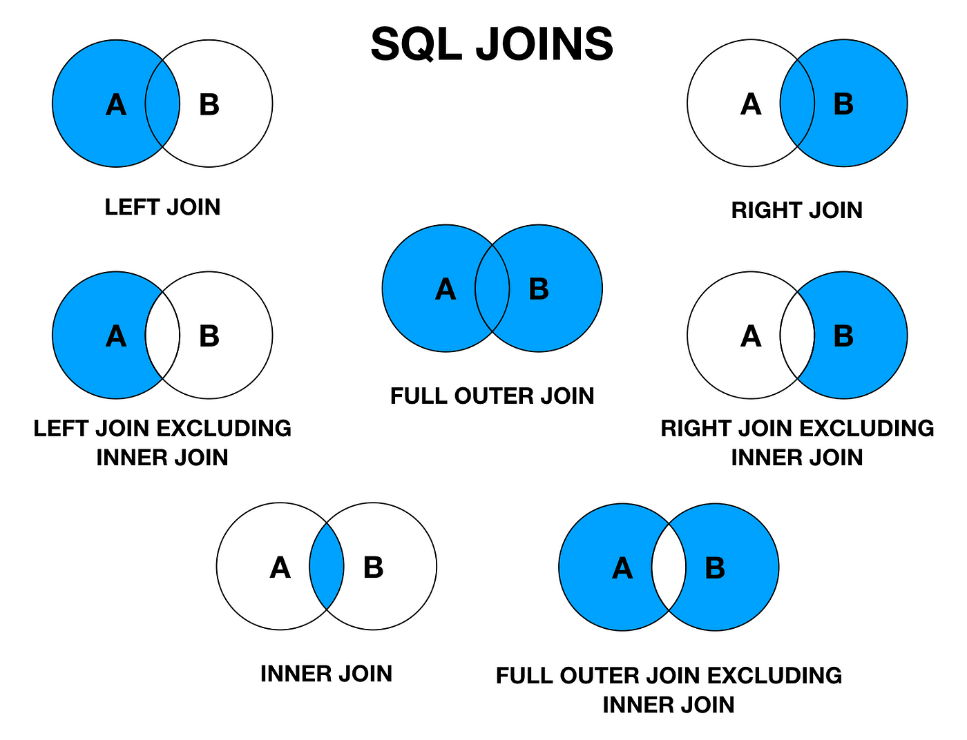
Practical Motivation (Early)
- Business questions span tables, not one table
- Examples you will actually run in PostgreSQL:
- Books with publisher name
- Books with author list (STRING_AGG)
- Publishers with zero books (quality)
- Store facts once, query them many times
-- Typical questions :
-- 1) Show each book with publisher name
-- 2) Show each book with author names
-- 3) Find missing relationships (orphans)
-- That is why JOIN exists.
Diagram: Normalization Creates the Need for Joins
duplicated names
facts stored once
to answer questions
From ERD Relationship to SQL Join
- ERD shows relationships between entities
- SQL tables store those relationships using keys
- One to Many: put FK on the many side
- Many to Many: create a bridge table
- Traditional habit: let the ERD guide the join path
ERD relationship
↓ (implement)
PK/FK columns
↓ (query)
JOIN ON keys
Diagram: One to Many (Publisher → Books)
ERD
Publisher 1 —— ∞ BookTables
publishers(publisher_id, name)books(book_id, title, publisher_id FK)
Join
books.publisher_id = publishers.publisher_idDiagram: Many to Many (Books ↔ Authors)
a.author_id = ba.author_id
Why Joins Exist
- Relational design keeps data normalized
- Joins answer questions across tables
- Example: books and authors live in different tables
- Traditional habit: avoid duplicated facts
-- PostgreSQL example question:
-- Show each book with its author name
-- Need:
-- books + authors + relationship (book_authors)
Book Domain Tables
- authors(author_id,..).
- publishers(publisher_id,...)
- books(book_id, publisher_id, ...)
- book_authors(book_id, author_id) many to many
CREATE TABLE authors (
author_id SERIAL PRIMARY KEY,
name TEXT NOT NULL,
country TEXT
);
CREATE TABLE publishers (
publisher_id SERIAL PRIMARY KEY,
name TEXT NOT NULL
);
CREATE TABLE books (
book_id SERIAL PRIMARY KEY,
title TEXT NOT NULL,
publisher_id INT REFERENCES publishers(publisher_id),
published_year INT NOT NULL,
price NUMERIC(10,2) NOT NULL
);
CREATE TABLE book_authors (
book_id INT REFERENCES books(book_id),
author_id INT REFERENCES authors(author_id),
PRIMARY KEY (book_id, author_id)
);Concept Diagram: Join as Matching Keys
Example Data: authors
| author_id | name | country |
|---|---|---|
| 1 | Ada Lovelace | UK |
| 2 | Alan Turing | UK |
| 3 | Grace Hopper | USA |
| 4 | Edsger Dijkstra | Netherlands |
Example Data: books
| book_id | title | publisher_id | published_year | price |
|---|---|---|---|---|
| 10 | Foundations of Computing | 100 | 2020 | 59.00 |
| 11 | Practical SQL Systems | 101 | 2019 | 49.50 |
| 12 | Algorithms the Classic Way | 100 | 2018 | 72.25 |
| 13 | Systems Thinking | NULL | 2021 | 39.99 |
Example Data: publishers
| publisher_id | name |
|---|---|
| 100 | Classic Press |
| 101 | Data House |
| 102 | Future Books |
Example Data: book_authors (Bridge)
| book_id | author_id |
|---|---|
| 10 | 1 |
| 10 | 2 |
| 11 | 3 |
| 12 | 4 |
Concept: INNER JOIN
- Keep only rows that match on both sides
- Unmatched rows are dropped
- Most common join in reporting
- Traditional habit: start with INNER to validate keys
INNER JOIN = intersection
A ∩ B
Only matching keys from both tables
Books with publisher name (INNER JOIN)
- Match books.publisher_id to publishers.publisher_id
- Books with publisher_id NULL will not appear
SELECT
b.book_id,
b.title,
p.name AS publisher
FROM books b
INNER JOIN publishers p
ON b.publisher_id = p.publisher_id
ORDER BY b.book_id;
Question: INNER JOIN removes rows when...
Pick the best statement:
- The left table has NULLs
- No matching key exists on the other side
- There are duplicate columns
- ORDER BY is missing
Concept: LEFT JOIN
- Keep all rows from the left table
- Match rows from the right table when possible
- Unmatched right side becomes NULL
- Traditional habit: use LEFT JOIN for coverage checks
LEFT JOIN = keep left
All A
Plus matching B
Else NULL for B
Keep all books, even without publisher
- Shows "Systems Thinking" even publisher_id is NULL
- Publisher fields become NULL when missing
SELECT
b.book_id,
b.title,
p.name AS publisher
FROM books b
LEFT JOIN publishers p
ON b.publisher_id = p.publisher_id
ORDER BY b.book_id;
LEFT JOIN: WHERE vs ON (Why Results Change)
Filter in WHERE (❌ risky)
SELECT
b.book_id,
b.title,
p.name AS publisher
FROM books b
LEFT JOIN publishers p
ON b.publisher_id = p.publisher_id
WHERE p.name = 'Classic Press'
ORDER BY b.book_id;
WHERE runs after the join. Rows where p.name is NULL are removed.
| book_id | title | publisher |
|---|---|---|
| 10 | Foundations of Computing | Classic Press |
| 12 | Algorithms the Classic Way | Classic Press |
⚠ Books without a publisher are gone.
LEFT JOIN behaves like INNER JOIN.
Filter in ON (✅ correct)
SELECT
b.book_id,
b.title,
p.name AS publisher
FROM books b
LEFT JOIN publishers p
ON b.publisher_id = p.publisher_id
AND p.name = 'Classic Press'
ORDER BY b.book_id;
Filter is applied during the join. Left rows are preserved.
| book_id | title | publisher |
|---|---|---|
| 10 | Foundations of Computing | Classic Press |
| 11 | Practical SQL Systems | NULL |
| 12 | Algorithms the Classic Way | Classic Press |
| 13 | Systems Thinking | NULL |
✔ All books remain.
✔ Publisher attached only when it matches.
Rule: WHERE vs ON in LEFT JOIN
- Filters in WHERE run after the join
- LEFT JOIN, WHERE on right table can erase NULL
- Put right side filters in ON for outer joins
LEFT JOIN then WHERE (right_col = ...)
can behave like INNER JOIN
Safer:
LEFT JOIN ... ON ... AND (right_col = ...)
Filter publisher name safely
- Keep all books, attach publisher when "Classic Press"
- Filter belongs in ON
SELECT
b.book_id,
b.title,
p.name AS publisher
FROM books b
LEFT JOIN publishers p
ON b.publisher_id = p.publisher_id
AND p.name = 'Classic Press'
ORDER BY b.book_id;
Question: In a LEFT JOIN, putting a right table filter in WHERE...
What can happen?
- It keeps all left rows always
- It may remove unmatched left rows
- It changes primary keys
- It forces GROUP BY
Concept: RIGHT JOIN
- Mirror of LEFT JOIN
- Keep all rows from the right table
- Less common because LEFT JOIN works
- Traditional habit: prefer LEFT JOIN for readability
RIGHT JOIN = keep right
Usually rewrite as LEFT JOIN
by swapping sides
Rewrite RIGHT JOIN as LEFT JOIN
- Same result, clearer reading
- Place the preserved table on the left
-- RIGHT JOIN form
SELECT p.name, b.title
FROM books b
RIGHT JOIN publishers p
ON b.publisher_id = p.publisher_id;
-- Preferred LEFT JOIN form
SELECT p.name, b.title
FROM publishers p
LEFT JOIN books b
ON b.publisher_id = p.publisher_id;
Concept: FULL OUTER JOIN
- Keep all rows from both sides
- Match when possible
- Unmatched fields become NULL on the missing side
- Useful for reconciliation reports
- Note: supported in PostgreSQL
FULL OUTER JOIN = union of keys
All A and all B
Match when possible
Else NULLs
Reconcile books and publishers (FULL OUTER JOIN)
- Books w/o publishers and publishers w/o books
- Common for data quality audits
SELECT
b.title,
p.name AS publisher
FROM books b
FULL OUTER JOIN publishers p
ON b.publisher_id = p.publisher_id
ORDER BY p.name, b.title;
FULL OUTER JOIN: Inputs and Result (Reconciliation)
Table A: books
| book_id | title | publisher_id |
|---|---|---|
| 10 | Foundations of Computing | 100 |
| 11 | Practical SQL Systems | 101 |
| 12 | Algorithms the Classic Way | 100 |
| 13 | Systems Thinking | NULL |
Book 13 has no publisher_id.
Table B: publishers
| publisher_id | name |
|---|---|
| 100 | Classic Press |
| 101 | Data House |
| 102 | Future Books |
Publisher 102 has no books.
Result: FULL OUTER JOIN
SELECT
b.title,
p.name AS publisher
FROM books b
FULL OUTER JOIN publishers p
ON b.publisher_id = p.publisher_id
ORDER BY p.name, b.title;
| title | publisher |
|---|---|
| Systems Thinking | NULL |
| Algorithms the Classic Way | Classic Press |
| Foundations of Computing | Classic Press |
| Practical SQL Systems | Data House |
| NULL | Future Books |
Both “missing sides” appear: book without publisher → publisher is NULL, publisher without books → title is NULL.
Concept: CROSS JOIN
- Every row from A paired with every row from B
- Creates a Cartesian product
- Can explode row counts fast
- Useful for generating combinations
- Risk if run by accident
CROSS JOIN = all combinations
Rows = |A| × |B|
CROSS JOIN: Inputs and Result (Cartesian Product)
Table A: authors (subset)
| author_id | name |
|---|---|
| 1 | Ada Lovelace |
| 2 | Alan Turing |
2 rows
Table B: publishers (subset)
| publisher_id | name |
|---|---|
| 100 | Classic Press |
| 101 | Data House |
| 102 | Future Books |
3 rows
Result: CROSS JOIN
SELECT
a.name AS author,
p.name AS publisher
FROM authors a
CROSS JOIN publishers p
ORDER BY a.name, p.name;
| author | publisher |
|---|---|
| Ada Lovelace | Classic Press |
| Ada Lovelace | Data House |
| Ada Lovelace | Future Books |
| Alan Turing | Classic Press |
| Alan Turing | Data House |
| Alan Turing | Future Books |
Cartesian product: rows = |A| × |B| = 2 × 3 = 6.
All author and publisher combinations (CROSS JOIN)
- This is usually not what you want for business queries
- Good for synthetic test data or matrix reports
SELECT
a.name AS author,
p.name AS publisher
FROM authors a
CROSS JOIN publishers p
ORDER BY a.name, p.name;
Concept: Many to Many via Bridge Table
- A book can have many authors
- An author can write many books
- Bridge table book_authors connects them
- Join through the bridge, not by guessing
authors ← book_authors → books
Two joins:
authors to bridge
bridge to books
Books with author names (bridge join)
- Join books to book_authors
- Join book_authors to authors
- Produces one row per (book, author)
SELECT
b.title,
a.name AS author
FROM books b
JOIN book_authors ba
ON ba.book_id = b.book_id
JOIN authors a
ON a.author_id = ba.author_id
ORDER BY b.title, a.name;
Pattern: Aggregate After Join
- Many to many joins can duplicate book rows
- Then you group to summarize
- Example: count authors per book
SELECT
b.title,
COUNT(*) AS author_count
FROM books b
JOIN book_authors ba
ON ba.book_id = b.book_id
GROUP BY b.title
ORDER BY author_count DESC, b.title;
Pattern: Aggregate After Join (Many to Many)
Table: books (subset)
| book_id | title |
|---|---|
| 10 | Foundations of Computing |
| 11 | Practical SQL Systems |
| 12 | Algorithms the Classic Way |
| 13 | Systems Thinking |
One row per book
Table: book_authors (bridge)
| book_id | author_id |
|---|---|
| 10 | 1 |
| 10 | 2 |
| 11 | 3 |
| 12 | 4 |
Many rows per book possible
Join duplicates, then GROUP BY summarizes
SELECT
b.title,
COUNT(*) AS author_count
FROM books b
JOIN book_authors ba
ON ba.book_id = b.book_id
GROUP BY b.title
ORDER BY author_count DESC, b.title;
Joined rows (one per book-author match)
| title | author_id |
|---|---|
| Foundations of Computing | 1 |
| Foundations of Computing | 2 |
| Practical SQL Systems | 3 |
| Algorithms the Classic Way | 4 |
Grouped result (one row per book)
| title | author_count |
|---|---|
| Foundations of Computing | 2 |
| Algorithms the Classic Way | 1 |
| Practical SQL Systems | 1 |
Question: Why can joins change counts?
After joining books to book_authors, book rows may appear multiple times because:
- JOIN always removes duplicates
- A book can match multiple bridge rows
- GROUP BY runs first
- ORDER BY creates extra rows
Pattern: Find Books Without Authors (LEFT JOIN)
- Data quality check
- Left join to bridge and filter unmatched
- Traditional habit: check for missing relationships
SELECT
b.book_id,
b.title
FROM books b
LEFT JOIN book_authors ba
ON ba.book_id = b.book_id
WHERE ba.book_id IS NULL
ORDER BY b.book_id;
Pattern: Find Books Without Authors (LEFT JOIN)
Table: books
| book_id | title |
|---|---|
| 10 | Foundations of Computing |
| 11 | Practical SQL Systems |
| 12 | Algorithms the Classic Way |
| 13 | Systems Thinking |
All books (starting point)
Table: book_authors
| book_id | author_id |
|---|---|
| 10 | 1 |
| 10 | 2 |
| 11 | 3 |
| 12 | 4 |
Bridge rows (missing book_id = 13)
LEFT JOIN + IS NULL (Anti Join)
SELECT
b.book_id,
b.title
FROM books b
LEFT JOIN book_authors ba
ON ba.book_id = b.book_id
WHERE ba.book_id IS NULL
ORDER BY b.book_id;
After LEFT JOIN (unmatched become NULL)
| book_id | title | ba.book_id |
|---|---|---|
| 10 | Foundations of Computing | 10 |
| 10 | Foundations of Computing | 10 |
| 11 | Practical SQL Systems | 11 |
| 12 | Algorithms the Classic Way | 12 |
| 13 | Systems Thinking | NULL |
Filtered result (books with no authors)
| book_id | title |
|---|---|
| 13 | Systems Thinking |
Traditional habit: LEFT JOIN + IS NULL reveals missing relationships.
Concept: Anti Join (Find Missing Matches)
- Anti join returns rows with no match
- Common as LEFT JOIN then IS NULL
- Also possible with NOT EXISTS
Anti join goal:
Keep A rows where no B match exists
Concept: Anti Join (Find Missing Matches)
Table A (books)
| book_id | title |
|---|---|
| 10 | Foundations of Computing |
| 11 | Practical SQL Systems |
| 12 | Algorithms the Classic Way |
| 13 | Systems Thinking |
We want books that have no match in Table B.
Table B (book_authors)
| book_id | author_id |
|---|---|
| 10 | 1 |
| 10 | 2 |
| 11 | 3 |
| 12 | 4 |
Missing match: book_id = 13
Anti Join Result
Goal: keep A rows where no B match exists.
-- Pattern 1 (common): LEFT JOIN then IS NULL
SELECT b.book_id, b.title
FROM books b
LEFT JOIN book_authors ba
ON ba.book_id = b.book_id
WHERE ba.book_id IS NULL
ORDER BY b.book_id;
-- Pattern 2 (also common): NOT EXISTS
SELECT b.book_id, b.title
FROM books b
WHERE NOT EXISTS (
SELECT 1
FROM book_authors ba
WHERE ba.book_id = b.book_id
)
ORDER BY b.book_id;
Result table
| book_id | title |
|---|---|
| 13 | Systems Thinking |
Traditional habit: use anti joins for data quality (missing links, orphan checks).
Books Without Authors (NOT EXISTS)
- Often clearer for complex keys
- Good habit: use EXISTS for yes or no questions
SELECT
b.book_id,
b.title
FROM books b
WHERE NOT EXISTS (
SELECT 1
FROM book_authors ba
WHERE ba.book_id = b.book_id
)
ORDER BY b.book_id;
Books Without Authors (NOT EXISTS)
Table: books
| book_id | title |
|---|---|
| 10 | Foundations of Computing |
| 11 | Practical SQL Systems |
| 12 | Algorithms the Classic Way |
| 13 | Systems Thinking |
- Often clearer for complex keys
- Good habit: use EXISTS for yes or no questions
Table: book_authors
| book_id | author_id |
|---|---|
| 10 | 1 |
| 10 | 2 |
| 11 | 3 |
| 12 | 4 |
Missing: book_id = 13 has no rows here.
Query + Result
SELECT
b.book_id,
b.title
FROM books b
WHERE NOT EXISTS (
SELECT 1
FROM book_authors ba
WHERE ba.book_id = b.book_id
)
ORDER BY b.book_id;
Result table
| book_id | title |
|---|---|
| 13 | Systems Thinking |
Traditional habit: use NOT EXISTS when you only need a yes/no match, not joined columns.
Concept: Semi Join (EXISTS)
- Return left rows that have at least one match
- Does not duplicate left rows
- Useful when only need books, not author columns
Semi join:
Keep A rows where a match exists in B
Use EXISTS
Concept: Semi Join (EXISTS)
Table A (books)
| book_id | title |
|---|---|
| 10 | Foundations of Computing |
| 11 | Practical SQL Systems |
| 12 | Algorithms the Classic Way |
| 13 | Systems Thinking |
- Return left rows that have at least one match
- Does not duplicate left rows
- Useful when you only need books, not author columns
Table B (book_authors)
| book_id | author_id |
|---|---|
| 10 | 1 |
| 10 | 2 |
| 11 | 3 |
| 12 | 4 |
Exists match for: 10, 11, 12
No match for: 13
Semi Join Result
Goal: keep A rows where a B match exists.
SELECT
b.book_id,
b.title
FROM books b
WHERE EXISTS (
SELECT 1
FROM book_authors ba
WHERE ba.book_id = b.book_id
)
ORDER BY b.book_id;
Result table
| book_id | title |
|---|---|
| 10 | Foundations of Computing |
| 11 | Practical SQL Systems |
| 12 | Algorithms the Classic Way |
Traditional habit: use EXISTS to avoid duplicates when the right side is “many”.
Books that have at least one author (EXISTS)
- Returns each qualifying book once
- No need for GROUP BY
SELECT
b.book_id,
b.title
FROM books b
WHERE EXISTS (
SELECT 1
FROM book_authors ba
WHERE ba.book_id = b.book_id
)
ORDER BY b.book_id;
Concept: SELF JOIN
- Join a table to itself
- Used for hierarchies and comparisons
- Requires table aliases
- Traditional habit: name aliases clearly
authors a1 JOIN authors a2
Same table, different roles
Self Join Example Table: editions
- editions(edition_id, ..., previous_edition_id)
- previous_edition_id references editions.edition_id
CREATE TABLE editions (
edition_id INT PRIMARY KEY,
book_id INT REFERENCES books(book_id),
edition_number INT NOT NULL,
previous_edition_id INT REFERENCES editions(edition_id)
);
Self Join Example: editions
- Table references itself
previous_edition_id → edition_id- Shows version chains
| edition_id | edition_number | previous_edition_id |
|---|---|---|
| 1 | 1 | NULL |
| 2 | 2 | 1 |
| 3 | 3 | 2 |
SELECT
e.edition_number,
prev.edition_number AS prev
FROM editions e
LEFT JOIN editions prev
ON e.previous_edition_id = prev.edition_id;
| edition | prev |
|---|---|
| 1 | NULL |
| 2 | 1 |
| 3 | 2 |
Show each edition with its previous edition
- Left join so first edition still appears
- Self join on previous_edition_id
SELECT
e.edition_id,
e.edition_number,
prev.edition_number AS previous_edition_number
FROM editions e
LEFT JOIN editions prev
ON e.previous_edition_id = prev.edition_id
ORDER BY e.edition_id;
Concept: Non Equi Join
- Join condition uses < > BETWEEN
- Common for ranges and bucketing
- Example: price bands table
JOIN ... ON b.price BETWEEN band.min AND band.max
Not just equality
Concept: Non Equi Join
- Join uses
< > BETWEEN - Common for ranges and buckets
- Example: price bands
| band | min | max |
|---|---|---|
| Budget | 0 | 39.99 |
| Standard | 40 | 69.99 |
| Premium | 70 | 999 |
SELECT
b.title,
pb.band
FROM books b
JOIN price_bands pb
ON b.price BETWEEN pb.min AND pb.max;
| title | band |
|---|---|
| Foundations of Computing | Standard |
| Algorithms the Classic Way | Premium |
| Systems Thinking | Budget |
Example Table: price_bands
- price_bands(band, min_price, max_price)
- Used to label books as Budget, Standard, Premium
CREATE TABLE price_bands (
band TEXT PRIMARY KEY,
min_price NUMERIC(10,2) NOT NULL,
max_price NUMERIC(10,2) NOT NULL
);
-- Example rows:
-- ('Budget', 0.00, 39.99)
-- ('Standard', 40.00, 69.99)
-- ('Premium', 70.00, 9999.99)
Assign each book a price band
- Join on a range condition
- Useful for reports and dashboards
SELECT
b.title,
b.price,
pb.band
FROM books b
JOIN price_bands pb
ON b.price BETWEEN pb.min_price AND pb.max_price
ORDER BY b.price DESC;
Concept: Joining 3 Tables Cleanly
- Join step by step
- Each ON should match a real relationship
- Traditional habit: one relationship per ON line
books → publishers
books → book_authors → authors
Keep each link explicit
Book, publisher, and author (multi join)
- Produces one row per (book, author)
- Publisher repeats per book
SELECT
b.title,
p.name AS publisher,
a.name AS author
FROM books b
LEFT JOIN publishers p
ON b.publisher_id = p.publisher_id
JOIN book_authors ba
ON ba.book_id = b.book_id
JOIN authors a
ON a.author_id = ba.author_id
ORDER BY b.title, a.name;
Concept: DISTINCT After Join
- Joins often create repeated values
- DISTINCT removes duplicate output rows
- Understand why duplicates happen first
If you want unique books only:
SELECT DISTINCT b.book_id, b.title
...
Concept: DISTINCT After Join
- Joins can duplicate rows
- Common in many to many joins
- DISTINCT removes repeated output rows
| book_id | title | author |
|---|---|---|
| 10 | Foundations of Computing | Ada |
| 10 | Foundations of Computing | Turing |
Same book appears multiple times.
SELECT DISTINCT
b.book_id,
b.title
FROM books b
JOIN book_authors ba
ON ba.book_id = b.book_id;
| book_id | title |
|---|---|
| 10 | Foundations of Computing |
One row per book.
Unique books that have at least one author
- Join returns many rows per book
- DISTINCT keeps each book once
SELECT DISTINCT
b.book_id,
b.title
FROM books b
JOIN book_authors ba
ON ba.book_id = b.book_id
ORDER BY b.book_id;
Concept: USING and NATURAL JOIN
- USING(column) for equality on same column
- NATURAL JOIN matches columns automatically
- Avoid NATURAL JOIN in production
- Reason: schema changes can silently change results
Prefer explicit ON
USING is acceptable if column names are stable
Avoid NATURAL JOIN
Concept: USING and NATURAL JOIN
- USING(column) = on same column name
- NATURAL JOIN matches same named columns
- USING is readable when schemas are stable
- Avoid NATURAL JOIN
| books | publishers |
|---|---|
| publisher_id | publisher_id |
-- Explicit (best)
JOIN publishers p
ON b.publisher_id = p.publisher_id
-- Shorthand
JOIN publishers p
USING (publisher_id)
-- Avoid
NATURAL JOIN publishers
Traditional habit: prefer explicit ON.
USING with publishers
- Works when both tables share same column name
- Still clearer than NATURAL JOIN
-- If both tables have publisher_id
SELECT
b.title,
p.name AS publisher
FROM books b
JOIN publishers p
USING (publisher_id);
Handling NULLs in Joined Output (COALESCE)
- Outer joins can produce NULLs on missing side
- COALESCE replaces NULL with a label
- Make missing values visible in reports
SELECT
b.title,
COALESCE(p.name, 'Unknown Publisher') AS publisher
FROM books b
LEFT JOIN publishers p
ON b.publisher_id = p.publisher_id;
Handling NULLs in Joined Output (COALESCE)
- Outer joins can produce NULLs
COALESCEreplaces NULL with a label- Makes missing data visible
| title | publisher |
|---|---|
| Foundations of Computing | Classic Press |
| Systems Thinking | NULL |
NULL hides missing information.
SELECT
b.title,
COALESCE(p.name, 'Unknown') AS publisher
FROM books b
LEFT JOIN publishers p
ON b.publisher_id = p.publisher_id;
| title | publisher |
|---|---|
| Foundations of Computing | Classic Press |
| Systems Thinking | Unknown |
Clear and explicit in reports.
Pattern: Filter Before Join (Reduce Rows)
- Smaller input can improve performance
- Filter books by year, then join
- Traditional habit: remove rows early when safe
SELECT b.title, p.name
FROM (
SELECT * FROM books
WHERE published_year >= 2020
) b
LEFT JOIN publishers p
ON b.publisher_id = p.publisher_id;
Pattern: Join Then Filter
- Sometimes you must join to filter
- Example: publishers named "Data House"
- Inner join is fine here
SELECT b.title, p.name
FROM books b
JOIN publishers p
ON b.publisher_id = p.publisher_id
WHERE p.name = 'Data House';
Rule: Qualify Column Names
- Joined tables often share column names like id, name
- Always use aliases: b.title, a.name, p.name
- Traditional habit: never rely on guessing
SELECT name
FROM books b
JOIN publishers p ON ...
-- Ambiguous: which name?
SELECT p.name
-- Clear
Traditional Habit: Read Joins Left to Right
- Start from the main table in FROM
- Add joins one by one
- Keep ON conditions near the join they describe
- Use consistent alias letters
FROM books b
LEFT JOIN publishers p ON ...
JOIN book_authors ba ON ...
JOIN authors a ON ...
One step at a time
Pitfall: COUNT(*) After a Many to Many Join
- COUNT(*) counts joined rows, not original entities
- To count books, use COUNT(DISTINCT b.book_id)
- Traditional habit: define what you are counting
SELECT
COUNT(*) AS joined_rows,
COUNT(DISTINCT b.book_id) AS unique_books
FROM books b
JOIN book_authors ba
ON ba.book_id = b.book_id;
Practice: Read This Join Query
SELECT
p.name AS publisher,
COUNT(*) AS book_rows
FROM publishers p
LEFT JOIN books b
ON b.publisher_id = p.publisher_id
GROUP BY p.name
ORDER BY book_rows DESC;
What is being counted?
- Authors per publisher
- Books per publisher including publishers with zero books
- Publishers per author
- Only publishers that have books
Pattern: One Row per Book with Author List
- Many to many produces multiple rows per book
- String aggregation makes a readable list
- PostgreSQL: STRING_AGG
SELECT
b.title,
STRING_AGG(a.name, ', ' ORDER BY a.name) AS authors
FROM books b
JOIN book_authors ba ON ba.book_id = b.book_id
JOIN authors a ON a.author_id = ba.author_id
GROUP BY b.title
ORDER BY b.title;
One Row per Book with Author List
- Many to many → multiple rows per book
- Hard to read in reports
- PostgreSQL:
STRING_AGG
| title | author |
|---|---|
| Foundations of Computing | Ada |
| Foundations of Computing | Turing |
Same book, many rows.
SELECT
b.title,
STRING_AGG(a.name, ', ' ORDER BY a.name) AS authors
FROM books b
JOIN book_authors ba ON ba.book_id = b.book_id
JOIN authors a ON a.author_id = ba.author_id
GROUP BY b.title
ORDER BY b.title;
| title | authors |
|---|---|
| Foundations of Computing | Ada, Turing |
One row, readable list.
Pattern: Top N Authors by Book Count
- Join through bridge
- Group by author
- Order and limit for ranking
SELECT
a.name,
COUNT(*) AS books_written
FROM authors a
JOIN book_authors ba
ON ba.author_id = a.author_id
GROUP BY a.name
ORDER BY books_written DESC, a.name
LIMIT 5;
Top N Authors by Book Count
- Join through bridge table
- Group by author
- Order + LIMIT for ranking
| author | book_id |
|---|---|
| Ada | 10 |
| Ada | 12 |
| Turing | 10 |
Bridge creates one row per (author, book).
SELECT
a.name,
COUNT(*) AS books_written
FROM authors a
JOIN book_authors ba
ON ba.author_id = a.author_id
GROUP BY a.name
ORDER BY books_written DESC, a.name
LIMIT 5;
| author | books_written |
|---|---|
| Ada | 2 |
| Turing | 1 |
Ranked summary.
Pattern: Recent Books with Authors
- Filter books by year
- Then join to show authors
- Traditional habit: keep the time filter clear
SELECT
b.title,
b.published_year,
a.name AS author
FROM books b
JOIN book_authors ba ON ba.book_id = b.book_id
JOIN authors a ON a.author_id = ba.author_id
WHERE b.published_year >= 2020
ORDER BY b.published_year DESC, b.title, a.name;
Recent Books with Authors
- Filter books by year
- Then join to authors
- Keep the time filter clear
| title | year |
|---|---|
| Systems Thinking | 2021 |
| Foundations of Computing | 2020 |
| Algorithms the Classic Way | 2018 |
Only years ≥ 2020 qualify.
SELECT
b.title,
b.published_year,
a.name AS author
FROM books b
JOIN book_authors ba ON ba.book_id = b.book_id
JOIN authors a ON a.author_id = ba.author_id
WHERE b.published_year >= 2020
ORDER BY b.published_year DESC, b.title, a.name;
| title | year | author |
|---|---|---|
| Systems Thinking | 2021 | Grace |
| Foundations of Computing | 2020 | Ada |
| Foundations of Computing | 2020 | Turing |
Filter first, then join.
Quality Check: Publishers With Zero Books
- Start from publishers
- Left join to books
- Keep groups where count is zero
SELECT
p.name,
COUNT(b.book_id) AS book_count
FROM publishers p
LEFT JOIN books b
ON b.publisher_id = p.publisher_id
GROUP BY p.name
HAVING COUNT(b.book_id) = 0
ORDER BY p.name;
Publishers With Zero Books
- Start from publishers
- LEFT JOIN to books
- Keep count = 0
| publisher | book_id |
|---|---|
| Classic Press | 10 |
| Data House | 11 |
| Future Books | NULL |
NULL means no matching book.
SELECT
p.name,
COUNT(b.book_id) AS book_count
FROM publishers p
LEFT JOIN books b
ON b.publisher_id = p.publisher_id
GROUP BY p.name
HAVING COUNT(b.book_id) = 0
ORDER BY p.name;
| publisher | book_count |
|---|---|
| Future Books | 0 |
Data quality check.
Question: Why COUNT(b.book_id) not COUNT(*) here?
In a LEFT JOIN from publishers to books, COUNT(*) would:
- Count only real books
- Count one row even when no book exists
- Return NULL always
- Require DISTINCT automatically
Rule: Wrong ON Condition Creates Wrong Data
- If ON is missing or incorrect, results may multiply
- This can look like valid data but it is not
- Traditional habit: sanity check row counts
-- Bad: missing ON creates cross join
SELECT b.title, p.name
FROM books b
JOIN publishers p;
-- Good: correct ON
SELECT b.title, p.name
FROM books b
JOIN publishers p
ON b.publisher_id = p.publisher_id;
Traditional Habit: Think About Join Performance
- Joins are faster when keys are indexed
- Primary keys are indexed by default in most systems
- Foreign keys often need indexes for join speed
- Use EXPLAIN to learn the plan
-- Example: index the FK for faster joins
CREATE INDEX idx_books_publisher_id
ON books(publisher_id);
EXPLAIN
SELECT b.title, p.name
FROM books b
JOIN publishers p
ON b.publisher_id = p.publisher_id;
Practice: Pick the Join Type
Goal: list all books, show publisher name when it exists.
- INNER JOIN
- LEFT JOIN
- CROSS JOIN
- NATURAL JOIN
Practice: Spot the Mistake
SELECT b.title, p.name
FROM books b
LEFT JOIN publishers p
ON b.publisher_id = p.publisher_id
WHERE p.name = 'Classic Press';
What is the risk?
- It becomes a CROSS JOIN
- It may remove books with no publisher
- It prevents indexes from working
- It forces FULL OUTER JOIN
Practice: Write the Bridge Join
Goal: show author names and the titles they wrote.
You must use book_authors.
SELECT
a.name,
b.title
FROM authors a
JOIN book_authors ba
ON ba.author_id = a.author_id
JOIN books b
ON b.book_id = ba.book_id
ORDER BY a.name, b.title;
Pattern: Find Orphaned Foreign Keys
- Orphan means FK value has no matching PK
- Left join from child to parent
- Filter where parent PK is NULL
-- Orphaned books.publisher_id
SELECT
b.book_id,
b.title,
b.publisher_id
FROM books b
LEFT JOIN publishers p
ON b.publisher_id = p.publisher_id
WHERE b.publisher_id IS NOT NULL
AND p.publisher_id IS NULL
ORDER BY b.book_id;
Pattern: Cheapest Book per Publisher
- Compute min price per publisher
- Join back to get the row
- Classic reporting technique
SELECT
p.name AS publisher,
b.title,
b.price
FROM publishers p
JOIN (
SELECT publisher_id, MIN(price) AS min_price
FROM books
WHERE publisher_id IS NOT NULL
GROUP BY publisher_id
) m
ON m.publisher_id = p.publisher_id
JOIN books b
ON b.publisher_id = m.publisher_id
AND b.price = m.min_price
ORDER BY p.name, b.title;
Rule: NULL Does Not Equal NULL
- Equality comparisons with NULL are unknown
- Outer joins missing matches via NULL output
- Traditional habit: do not join on nullable text keys
NULL = NULL is not true
Prefer PK and FK joins
Avoid joining by names
Quick Review: Join Types and Use Cases
- INNER: matching rows only
- LEFT: keep all left rows
- RIGHT: keep all right rows
- FULL: keep all rows from both
- CROSS: all combinations
- SELF: table joins itself
Traditional habit:
Write joins so a reader can verify keys
without guessing
Practice Prompts
- List all books with publisher name, Unknown if NULL
- List authors who wrote at least two books
- Find publishers with zero books
- Show each book with a comma separated author list
- Find books that have no authors linked
Traditional habit: start with the join keys, then refine.
-- Template
SELECT ...
FROM ...
JOIN ... ON ...
LEFT JOIN ... ON ...
WHERE ...
GROUP BY ...
HAVING ...
ORDER BY ...
LIMIT ...;
Agenda Today
- Practice: Hiking registration system
- Review: Homework 1 and Lab 1 results
- Prepare: Homework 3 and Lab 3 (published)
- Prepare: Project Part 1 (published this afternoon)

Create Table: trail
- Primary key: trail_id
- Trail attributes
- capacity used later in HAVING
CREATE TABLE trail (
trail_id SERIAL PRIMARY KEY,
name TEXT NOT NULL,
difficulty TEXT NOT NULL,
capacity INT NOT NULL
);
Create Table: reservation
- Primary key: reservation_id
- Foreign key: trail_id
- One trail → many reservations
CREATE TABLE reservation (
reservation_id SERIAL PRIMARY KEY,
hiker_name TEXT NOT NULL,
hike_date DATE NOT NULL,
trail_id INT REFERENCES trail(trail_id)
);
Relationship
- Foreign key enforces integrity
- JOIN connects both tables
- Foundation of relational systems
trail (1) -------- (many) reservation
r.trail_id = t.trail_id
Practice 1 – Basic JOIN
- Show reservation_id
- Show hiker_name
- Show hike_date
- Show trail_name
Write an INNER JOIN
between reservation and trail.
Practice 2 – JOIN with Filter
- Only difficulty = 'Hard'
- Filter after JOIN
Add a WHERE clause.
Practice 3 – LEFT JOIN
- Show all trails
- Even without reservations
- Expect NULL values
Which JOIN keeps
all rows from trail?
Practice 4 – GROUP BY
- Count reservations per trail
- Return trail_name
- Return total_reservations
Use COUNT()
Use GROUP BY
Practice 5 – HAVING
- Find overbooked trails
- Definition: COUNT > capacity
Use GROUP BY
Use HAVING
Practice 6 – COUNT Only
- How many total reservations exist?
- No JOIN needed
Use COUNT(*)
Practice 7 – LIMIT
- Show first 3 reservations
- Ordered by hike_date
Use ORDER BY
Use LIMIT
Practice 8 – OFFSET
- Skip first 3 reservations
- Show next 3
Use LIMIT
Use OFFSET
Answer 1 – Basic JOIN
- Classic INNER JOIN
SELECT
r.reservation_id,
r.hiker_name,
r.hike_date,
t.name AS trail_name
FROM reservation r
JOIN trail t
ON r.trail_id = t.trail_id;
Answer 2 – JOIN with Filter
- Filter after JOIN
SELECT
r.hiker_name,
r.hike_date,
t.name AS trail_name
FROM reservation r
JOIN trail t
ON r.trail_id = t.trail_id
WHERE t.difficulty = 'Hard';
Answer 3 – LEFT JOIN
- All trails, even without reservations
SELECT
t.trail_id,
t.name AS trail_name,
r.reservation_id,
r.hiker_name,
r.hike_date
FROM trail t
LEFT JOIN reservation r
ON r.trail_id = t.trail_id
ORDER BY t.trail_id, r.hike_date;
Answer 4 – GROUP BY
- Aggregation per trail
SELECT
t.trail_id,
t.name AS trail_name,
COUNT(r.reservation_id) AS total_reservations
FROM trail t
LEFT JOIN reservation r
ON r.trail_id = t.trail_id
GROUP BY t.trail_id, t.name
ORDER BY total_reservations DESC, t.trail_id;
Answer 5 – HAVING
- Filter after aggregation
- Find overbooked trails
SELECT
t.trail_id,
t.name AS trail_name,
t.capacity,
COUNT(r.reservation_id) AS total_reservations
FROM trail t
LEFT JOIN reservation r
ON r.trail_id = t.trail_id
GROUP BY t.trail_id, t.name, t.capacity
HAVING COUNT(r.reservation_id) > t.capacity
ORDER BY total_reservations DESC, t.trail_id;
Answer 6 – COUNT Only
- Total rows in reservation
SELECT COUNT(*) AS total_reservations
FROM reservation;
Answer 7 – LIMIT
- First page of results
SELECT
reservation_id,
hiker_name,
hike_date,
trail_id
FROM reservation
ORDER BY hike_date, reservation_id
LIMIT 3;
Answer 8 – LIMIT + OFFSET
- Second page of results
- Skip 3, take 3
SELECT
reservation_id,
hiker_name,
hike_date,
trail_id
FROM reservation
ORDER BY hike_date, reservation_id
LIMIT 3 OFFSET 3;
Extra Practice – Aggregates
- MIN capacity
- MAX capacity
- AVG capacity
- Count trails per difficulty
Write 2 queries:
1) MIN/MAX/AVG on trail.capacity
2) GROUP BY trail.difficulty with COUNT(*)
Extra Answers – Aggregates
- Aggregate functions are built in
- Use GROUP BY for categories
-- 1) capacity stats
SELECT
MIN(capacity) AS min_capacity,
MAX(capacity) AS max_capacity,
AVG(capacity) AS avg_capacity
FROM trail;
-- 2) trails per difficulty
SELECT
difficulty,
COUNT(*) AS trails_count
FROM trail
GROUP BY difficulty
ORDER BY trails_count DESC;
Homework 1: Why is SQL Important?
- Standard language for relational databases
- Used across industries and systems
- Separates data storage from application logic
- Allows structured querying and reporting
- Foundation for analytics and decision making
In simple terms:
SQL is important because it gives us
a reliable and consistent way to
store, retrieve, and manage data.
Without SQL, structured data systems
would not scale or communicate well.
Homework 1: SQL vs SQLite
- SQL is a language
- SQLite is a database engine
- SQL defines the rules for querying data
- SQLite executes those SQL commands
- SQLite is lightweight and file based
SQL:
Structured Query Language
Standard for relational databases.
SQLite:
A software system that
implements SQL.
Language ≠ Database
Homework 1: CREATE
- Defines new database objects
- Creates tables, indexes, views
- Establishes structure before data
- Defines columns and constraints
CREATE TABLE students (
student_id INTEGER PRIMARY KEY,
name TEXT NOT NULL,
major TEXT
);
Homework 1: SELECT
- Retrieves data from tables
- Can filter with WHERE
- Can group with GROUP BY
- Can sort with ORDER BY
SELECT name, major
FROM students
WHERE major = 'CS';
Homework 1: INSERT
- Adds new rows to a table
- Must match defined structure
- Respects constraints
INSERT INTO students (student_id, name, major)
VALUES (1, 'Ana', 'CS');
Homework 1: UPDATE
- Modifies existing data
- Uses WHERE to target rows
- Without WHERE, affects all rows
UPDATE students
SET major = 'Data Science'
WHERE student_id = 1;
Homework 1: DELETE
- Removes rows from a table
- Should be used carefully
- Often restricted by foreign keys
DELETE FROM students
WHERE student_id = 1;
Homework 1: Syllabus Questions and Clarifications
| Student Question | Instructor Response |
|---|---|
| How are attendance and participation points calculated, and is there a maximum? | Attendance and participation are calculated based on consistent presence and meaningful engagement. |
| For team projects, how are individual contributions evaluated within a single team grade? | There is one overall team project grade, but each submission must clearly state individual responsibilities, and contributions may be reviewed through GitHub activity and documentation, with adjustments made if significant imbalance is observed. |
| Clarification on grading breakdown: What are the percentage values for labs, homework, projects, and exams? | The grading breakdown is as follows: Labs 15 percent, Homework 15 percent, Projects 40 percent, and Exams 30 percent. |
| How is assignment submission on GitHub acknowledged and recorded? | Assignment submission on GitHub is acknowledged by confirming that the code has been uploaded to the repository. |
Lab 1 – ERD 1
- Pros
- Identifies main entities clearly
- Shows attributes and constraints
- Basic relationship direction is correct
- Cons
- No named relationship
- No primary keys highlighted

Lab 1 – ERD 2
- Pros
- Primary keys introduced
- Named relationships
- Cons
- Still missing attributes
- E-Mail NOT NUll maybe too strict

Lab 1 – ERD 3
- Pros
- Attributes added to each entity
- Named relationship
- Cons
- Email NOT NULL maybe too strict

Lab 1 – ERD 4
- Pros
- Data types defined
- Named relationships
- Support for multiple libraries
- Cons
- No UNIQUE; NOT NULL; DEFAULT; CHECK constraints

Lab 1 – ERD 5
- Pros
- Data types defined
- Named relationships
- Email optional
- Cons
- Optional description attribute

Lab 1 – ERD 6
- Pros
- Primary and foreign keys defined
- Constraints included (NOT NULL, UNIQUE)
- Clearly models member borrows book
- Loan table connects entities correctly
- Cons
- Table name lower case

Lab 3: Relational Algebra and Advanced SQL (Due: Feb/27)
- Relational Algebra (Module 3)
- Database Interface (Module 4)
- Advanced SQL (Module 5)
- Write queries carefully
- Use uppercase SQL keywords
- Add semicolons after each query
Relational Algebra: Selection and Projection
- Relation: Flowers(flowerID, name, etc)
- Retrieve name and price
- Condition: red flowers
- Condition: stockQuantity > 20
Relational Algebra: Join (⨝)
- Relations: Flowers and Orders
- Match on flowerID
- Return flower names
- At least one order exists
Relational Algebra Optimization
- Identify inefficiency in join order
- Push selection earlier
- Reduce intermediate results
- Rewrite optimized expression
API and Database Interaction
- REST endpoint: GET /api/flowers?color=red
- Explain backend flow
- Describe SQL likely executed
- Think request → query → response
Web vs Console Interface
- One advantage web interface
- One disadvantage web interface
- One advantage SQL console
- One disadvantage SQL console
GROUP BY and Aggregation
- Average price grouped by category
- Use GROUP BY
- Filter grouped results
- With HAVING clause
CHECK Constraints
- Add 3 valid CHECK constraints
- Consider numeric limits
- Consider non negative values
- Consider domain restrictions
INNER JOIN
- Retrieve flowers with suppliers
- Match supplier_id
- Return related records only
LEFT JOIN
- Retrieve all customers
- Include orders if available
- Preserve unmatched customers
RIGHT JOIN
- Retrieve all products
- Include sales if available
- Preserve unmatched products
Homework 3: Joins, GROUP BY, CHECK (Due: TBD)
- Textbook 1: SQL The Complete Reference
- Textbook 2: Guide to SQLite
- Focus: Joins, performance, grouping, constraints
- Answer in your own words
- Be specific and concrete
- Reference the page number
Natural Join Risk (Textbook 1, p.128)
- Explain one risk of using NATURAL JOIN
- Hint: unintended matching columns
- Hint: schema changes over time
- Give a concrete example scenario
Which queries typically require JOINS? (Textbook 1, p.141)
- Explain when a JOIN is needed
- Hint: data split across tables
- Hint: one to many relationships
- Name common query types that need joins
Unmatched rows and OUTER JOIN (Textbook 1, p.149, Fig 7-12)
- Define what unmatched rows are
- Explain why they occur
- Explain how OUTER JOIN keeps them
- Mention what appears as NULL
GROUP BY query difference (Textbook 2, p.67–71)
- Compare the two provided queries
- Explain GROUP BY output level
- Explain HAVING as group filter
- State what changes in the result set
CHECK constraints meaning (Textbook 2, p.99)
- Interpret the sentence in plain language
- Explain what “modification” refers to
- Explain constraint evaluation true or false
- Give a simple example of failure
Submission guidance
- Write concise paragraphs
- Use clear examples
- Do not copy the textbook wording
- Show understanding, not memorization
Project: Plant Watering Database System
- Build a simple web application
- Track plant watering status
- Use Flask + PostgreSQL or SQLite
- Connect backend to web client
- Database design
- REST API development
- Frontend integration
- Team collaboration
- Teams of 3 (Frontend, Backend, Database)
- Choose unique team folder
- Work only inside your directory
- One shared PDF submission
- Upload to GitHub team-X/
- Submit teamX.pdf
- Include team number
- Include all member names
- Clone base project
- Use as Flask server template
- Copy code structure
- Do not modify original repo
git clone https://github.com/SE4CPS/2026-COMP-163.git
cd Project/Part-1/Sample
- Use team-specific table name
- Create flowers table
- Insert sample data
- Track watering status
- id (Primary Key)
- name
- last_watered
- water_level
- min_water_required
- GET all flowers
- GET flowers needing water
- POST new flower
- PUT update flower
- DELETE flower
- Use correct SQL queries
- Connect to database
- Return JSON response
- Test endpoints carefully
- Fetch data from /flowers
- Display table
- Show water status
- Yes or No indicator
- Use JavaScript fetch()
- Parse JSON
- Dynamically build rows
- Verify correct display
- Each plant loses 5 inches per day
- Use SQL UPDATE statement
- Calculate days since last_watered
- Simulate daily loss
UPDATE teamX_flowers
SET water_level =
water_level - (5 * (CURRENT_DATE - last_watered));
- Test API and frontend
- Upload to GitHub by March 21
- Add screenshots to PDF
- Prepare 5 minute presentation
- team-X/ GitHub directory
- Database table with data
- Flask API (app.py)
- Web client (flowers.html)
- Watering algorithm
- teamX.pdf
Normalization: Focus on 1NF
- Start from unnormalized operational data
- Remove repeating groups
- Make rows predictable
- Foundation for later normal forms
- Target
- One fact per cell
- One row per fact
- Clear primary key
Current Process
1970 – Before and After the Relational Model
Data in flat files Application specific formats Repeated fields Lists inside records
Hard to query Hard to integrate
Introduced the Relational Model
Data must fit into tables, rows, columns
Normalize data so SQL can query it
Unnormalized Data (UNF)
UNF Example: Orders with Lists
| order_id | customer | items | prices |
|---|---|---|---|
| 1001 | Alice | Rose,Tulip | 12.50,6.00 |
| 1002 | Bob | Lily,Orchid | 9.25,15.00 |
-- Not reliable in UNF SELECT * FROM Orders WHERE items = 'Rose';
Why Lists Break Queries
- Cannot count items by row
- Cannot FK to Flowers table
- String parsing required
- No type enforcement per item
-- Hacky and unsafe SELECT * FROM Orders WHERE items LIKE '%Rose%';
1NF Fix: One Row per Item
| order_id | flower | unit_price |
|---|---|---|
| 1001 | Rose | 12.50 |
| 1001 | Tulip | 6.00 |
| 1002 | Lily | 9.25 |
| 1002 | Orchid | 15.00 |
SELECT * FROM OrderItems WHERE flower = 'Rose';
1NF Rules
- Atomic values only
- No repeating groups
- No arrays or CSV inside cells
- Primary key defined
UNF Example: Multiple Phones
| customer | phones |
|---|---|
| Alice | 0101,0109 |
| Clara | 0103,0111 |
-- Impossible to enforce uniqueness SELECT COUNT(*) FROM Customers WHERE phones = '0101';
1NF Fix: CustomerPhones Table
| customer | phone |
|---|---|
| Alice | 0101 |
| Alice | 0109 |
| Clara | 0103 |
| Clara | 0111 |
SELECT * FROM CustomerPhones WHERE phone = '0101';
UNF: Combined City and State
| supplier | location |
|---|---|
| BloomCo | Stockton,CA |
| FloraSupreme | Sacramento,CA |
-- Cannot filter by state safely SELECT * FROM Suppliers WHERE location LIKE '%CA';
1NF Fix: Separate City and State
| supplier | city | state |
|---|---|---|
| BloomCo | Stockton | CA |
| FloraSupreme | Sacramento | CA |
SELECT * FROM Suppliers WHERE state = 'CA';
UNF: JSON Array in Column
| order_id | tags |
|---|---|
| 1001 | ["gift","red"] |
| 1002 | ["wedding"] |
-- Hard to count per tag SELECT COUNT(*) FROM Orders WHERE tags = 'gift';
1NF Fix: OrderTags Rows
| order_id | tag |
|---|---|
| 1001 | gift |
| 1001 | red |
| 1002 | wedding |
SELECT COUNT(*) FROM OrderTags WHERE tag = 'gift';
Missing Primary Key Causes Ambiguity
| order_id | flower |
|---|---|
| 1001 | Rose |
| 1001 | Rose |
-- Which row is correct? DELETE FROM OrderItems WHERE order_id = 1001 AND flower = 'Rose';
Correct Key in 1NF
| PK | PK |
|---|---|
| order_id | flower |
| 1001 | Rose |
| 1001 | Tulip |
Primary Key → (order_id, flower)
Step 1: UNF → Add Rows
| order_id | items | prices |
|---|---|---|
| 1001 | Rose,Tulip | 12.50,6.00 |
| 1002 | Lily,Orchid | 9.25,15.00 |
| order_id | items | prices |
|---|---|---|
| 1001 | Rose | 12.50 |
| 1001 | Tulip | 6.00 |
| 1002 | Lily | 9.25 |
| 1002 | Orchid | 15.00 |
Step 2: Atomic Values → Add Columns
| supplier | address |
|---|---|
| BloomCo | 123 Market, Stockton, CA |
| FloraSupreme | 45 Garden, Sacramento, CA |
| supplier | street | city | state |
|---|---|---|---|
| BloomCo | 123 Market | Stockton | CA |
| FloraSupreme | 45 Garden | Sacramento | CA |
| PK | PK | |
|---|---|---|
| order_id | flower | unit_price |
| 1001 | Rose | 12.50 |
| 1001 | Tulip | 6.00 |
| 1002 | Lily | 9.25 |
| 1002 | Orchid | 15.00 |
Summary
- 1NF removes repeating groups
- Each cell atomic
- Each row identifiable
- Queries become relational
Example: Hiking Reservation Data (UNF)
reservation_id | hiker_name | trails | dates --------------------------------------------------------------------------- 5001 | Alice | Half Dome, Full Day | 2026-06-01, 2026-06-02 5001 | Bob | Yosemite Falls, Morning | 2026-06-03 5002 | Clara | Half Dome, Yosemite Falls | 2026-06-04, 2026-06-05 5002 | Tom | Mist Trail | 2026-06-06
Goal: Transform this data to 1NF
- No lists - Atomic value - Primary key
2nd Normal Form (2NF)
- 1NF achieved
- Next: remove partial dependencies
- Then: remove transitive dependencies
Normalization: Focus on 2NF
- Start from a table that is already 1NF
- Composite key creates the risk
- Remove partial dependency
- Order facts should not repeat per item row
- Target
- Non key columns depend on the full key
- No column depends only on order_id
- No column depends only on flower
2NF Before: 1NF Table with Composite Key
| PK | PK | |||
|---|---|---|---|---|
| order_id | flower | unit_price | customer | phone |
| 1001 | Rose | 12.50 | Alice | 0101 |
| 1001 | Tulip | 6.00 | Alice | 0101 |
| 1002 | Lily | 9.25 | Bob | 0102 |
| 1002 | Orchid | 15.00 | Bob | 0102 |
-- Update touches multiple rows (symptom) UPDATE OrderItems SET phone = '9999' WHERE order_id = 1001;
2NF Problem: Partial Dependency
| Column | Depends on | Why this is bad |
|---|---|---|
| customer | order_id | Repeats per item row |
| phone | order_id | Repeats per item row |
| unit_price | flower | Repeats across many orders |
- Key is (order_id, flower)
- But customer, phone depend only on order_id
- And unit_price depends only on flower
- 2NF fix is to split by dependency
2NF Fix 1: Move Order Facts to Orders
| PK | ||
|---|---|---|
| order_id | customer | phone |
| 1001 | Alice | 0101 |
| 1002 | Bob | 0102 |
| PK | |||
|---|---|---|---|
| order_item_id | order_id | flower | unit_price |
| 1 | 1001 | Rose | 12.50 |
| 2 | 1001 | Tulip | 6.00 |
| 3 | 1002 | Lily | 9.25 |
| 4 | 1002 | Orchid | 15.00 |
-- Phone changes once UPDATE Orders SET phone = '9999' WHERE order_id = 1001;
2NF Fix 2: Move Flower Facts to Flowers
| PK | ||
|---|---|---|
| flower_id | name | list_price |
| 1 | Rose | 12.50 |
| 2 | Tulip | 6.00 |
| 3 | Lily | 9.25 |
| 4 | Orchid | 15.00 |
| PK | ||
|---|---|---|
| order_item_id | order_id | flower_id |
| 1 | 1001 | 1 |
| 2 | 1001 | 2 |
| 3 | 1002 | 3 |
| 4 | 1002 | 4 |
-- Price changes once UPDATE Flowers SET list_price = 13.00 WHERE flower_id = 1;
2NF Result
- Orders holds order facts
- Flowers holds flower facts
- OrderItems holds links only
- No partial dependency remains
- Keys
- Orders: order_id
- Flowers: flower_id
- OrderItems: order_item_id
Normalization: Focus on 3NF
- Start from tables that are already 2NF
- Remove transitive dependency
- Non key columns independent of non key columns
- Supplier details are the classic example
- Target
- Key → non key only
- Not: key → non key → non key
- Supplier facts stored once
3NF Before: Supplier Facts Inside Flowers
| PK | ||||
|---|---|---|---|---|
| flower_id | name | list_price | supplier_name | supplier_addr |
| 1 | Rose | 12.50 | BloomCo | 123 Market |
| 2 | Tulip | 6.00 | BloomCo | 123 Market |
| 3 | Lily | 9.25 | FloraSupreme | 45 Garden |
| 4 | Orchid | 15.00 | FloraSupreme | 45 Garden |
-- Update anomaly (address repeated) UPDATE Flowers SET supplier_addr = '125 Market' WHERE supplier_name = 'BloomCo';
Transitive Dependency
A transitive dependency occurs when a non key attribute depends on another non key attribute instead of directly on the primary key.3NF Fix: Create Suppliers and Reference by Key
| PK | |||
|---|---|---|---|
| supplier_id | name | street | city |
| 10 | BloomCo | 123 Market | Stockton |
| 20 | FloraSupreme | 45 Garden | Sacramento |
| PK | |||
|---|---|---|---|
| flower_id | name | list_price | supplier_id |
| 1 | Rose | 12.50 | 10 |
| 2 | Tulip | 6.00 | 10 |
| 3 | Lily | 9.25 | 20 |
| 4 | Orchid | 15.00 | 20 |
-- Address changes once UPDATE Suppliers SET street = '125 Market' WHERE supplier_id = 10;
3NF Result: Clean Join for Orders
| PK | ||
|---|---|---|
| order_item_id | order_id | flower_id |
| 1 | 1001 | 1 |
| 2 | 1001 | 2 |
| 3 | 1002 | 3 |
| 4 | 1002 | 4 |
SELECT o.order_id, o.customer, f.name, s.name AS supplier FROM Orders o JOIN OrderItems oi ON oi.order_id = o.order_id JOIN Flowers f ON f.flower_id = oi.flower_id JOIN Suppliers s ON s.supplier_id = f.supplier_id;
3NF Summary
- Moved supplier facts to Suppliers
- Flowers stores only supplier key
- Eliminated transitive dependency
- Updates happen in one place
- Final tables
- Orders(order_id)
- OrderItems(order_item_id)
- Flowers(flower_id)
- Suppliers(supplier_id)
After 1NF
| PK | PK | |||||
|---|---|---|---|---|---|---|
| order_id | flower | customer | phone | unit_price | supplier_name | supplier_addr |
| 1001 | Rose | Alice | 0101 | 12.50 | BloomCo | 123 Market |
| 1001 | Tulip | Alice | 0101 | 6.00 | BloomCo | 123 Market |
| 1002 | Lily | Bob | 0102 | 9.25 | FloraSupreme | 45 Garden |
| 1002 | Orchid | Bob | 0102 | 15.00 | FloraSupreme | 45 Garden |
After 2NF
| PK | ||
|---|---|---|
| order_id | customer | phone |
| 1001 | Alice | 0101 |
| 1002 | Bob | 0102 |
| PK | PK | |||
|---|---|---|---|---|
| order_id | flower | unit_price | supplier_name | supplier_addr |
| 1001 | Rose | 12.50 | BloomCo | 123 Market |
| 1001 | Tulip | 6.00 | BloomCo | 123 Market |
| 1002 | Lily | 9.25 | FloraSupreme | 45 Garden |
| 1002 | Orchid | 15.00 | FloraSupreme | 45 Garden |
After 3NF
| PK | ||
|---|---|---|
| supplier_id | name | addr |
| 10 | BloomCo | 123 Market |
| 20 | FloraSupreme | 45 Garden |
Flowers
| PK | ||
|---|---|---|
| flower_id | name | supplier_id |
| 1 | Rose | 10 |
| 2 | Tulip | 10 |
| 3 | Lily | 20 |
| 4 | Orchid | 20 |
| PK | ||
|---|---|---|
| order_id | customer | phone |
| 1001 | Alice | 0101 |
| 1002 | Bob | 0102 |
OrderItems
| PK | PK | |
|---|---|---|
| order_id | flower_id | unit_price |
| 1001 | 1 | 12.50 |
| 1001 | 2 | 6.00 |
| 1002 | 3 | 9.25 |
| 1002 | 4 | 15.00 |
Normal Forms and Storage Cost Over Time
| Year | Normal Form |
|---|---|
| 1970 | 1NF |
| 1971 | 2NF |
| 1971 | 3NF |
| Year | ~Cost per MB |
|---|---|
| 1970 | $1,000,000+ |
| 1980 | $10,000 |
| 1990 | $100 |
| 2000 | $1 |
| 2010 | $0.10 |
| 2020 | <$0.02 |
Today: Storage Is Cheap
32 GB = 32,000 MB
Cost per MB:
10 / 32,000 ≈ 0.0003 $
Less than 1/1000 of a cent per MB

32GB SD Card
Normalization Is About Accuracy
Supplier address stored in many rows
Change address → update 20 rows
Miss 1 row → Inconsistent data
Supplier stored once
Change address → update 1 row
No update anomaly
DBMS Enforces 1NF Basics
PRIMARY KEY
| Constraint | Works on Atomic Value? |
|---|---|
| PRIMARY KEY | Yes |
| UNIQUE | Yes |
| NOT NULL | Yes |
| CHECK | Yes |
| FOREIGN KEY | Yes |
Lists like "Rose,Tulip" cannot be validated properly
Normalization Process
NF1 Practice – Question 1
Which columns violate 1NF?
Why?
reservation_id | hiker_name | trails | dates
---------------------------------------------------------------------------
5001 | Alice | Half Dome, Mist Trail | 2026-06-01, Feb
5001 | Bob | Yosemite Falls | 2026-06-03
5002 | Clara | Half Dome, Yosemite Falls | 2026-06-04, Apr
5002 | Tom | Mist Trail | 2026-06-06
NF1 Practice – Question 2
How would you remove the repeating groups?
What should become rows?
reservation_id | hiker_name | trails | dates
---------------------------------------------------------------------------
5001 | Alice | Half Dome, Mist Trail | 2026-06-01, Dec
5001 | Bob | Yosemite Falls | 2026-06-03
5002 | Clara | Half Dome, Yosemite Falls | 2026-06-04, Feb
5002 | Tom | Mist Trail | 2026-06-06
NF1 Practice – Question 3
After removing lists, what should the primary key be?
Is reservation_id enough?
reservation_id | hiker_name | trails | dates
---------------------------------------------------------------------------
5001 | Alice | Half Dome, Mist Trail | 2026-06-01, Jan
5001 | Bob | Yosemite Falls | 2026-06-03
5002 | Clara | Half Dome, Yosemite Falls | 2026-06-04, Apr
5002 | Tom | Mist Trail | 2026-06-06
NF1 Practice – Question 4
Can this table enforce UNIQUE or FOREIGN KEY constraints correctly?
Why or why not?
reservation_id | hiker_name | trails | dates
---------------------------------------------------------------------------
5001 | Alice | Half Dome, Mist Trail | 2026-06-01, Feb
5001 | Bob | Yosemite Falls | 2026-06-03
5002 | Clara | Half Dome, Yosemite Falls | 2026-06-04, Mar
5002 | Tom | Mist Trail | 2026-06-06
NF1 Practice – Question 5
Rewrite this dataset in proper 1NF form.
Define:
- Columns - Rows - Primary Key
reservation_id | hiker_name | trails | dates
---------------------------------------------------------------------------
5001 | Alice | Half Dome, Mist Trail | 2026-06-01, Feb
5001 | Bob | Yosemite Falls | 2026-06-03
5002 | Clara | Half Dome, Yosemite Falls | 2026-06-04, Apr
5002 | Tom | Mist Trail | 2026-06-06
Agenda Today
- Practice: Hiking registration system
- Review: Homework 3 and Lab 3 (published)
- Review: Project Part 1 (published)
Create Table: trail
- Primary key: trail_id
- Trail attributes
- capacity used later in HAVING
CREATE TABLE trail (
trail_id SERIAL PRIMARY KEY,
name TEXT NOT NULL,
difficulty TEXT NOT NULL,
capacity INT NOT NULL
);
Create Table: reservation
- Primary key: reservation_id
- Foreign key: trail_id
- One trail → many reservations
CREATE TABLE reservation (
reservation_id SERIAL PRIMARY KEY,
hiker_name TEXT NOT NULL,
hike_date DATE NOT NULL,
trail_id INT REFERENCES trail(trail_id)
);
Relationship
- Foreign key enforces integrity
- JOIN connects both tables
- Foundation of relational systems
trail (1) -------- (many) reservation
r.trail_id = t.trail_id
Practice 1 – Basic JOIN
- Show reservation_id
- Show hiker_name
- Show hike_date
- Show trail_name
Write an INNER JOIN
between reservation and trail.
Integrate Existing Data
- Primary key: trail_id
- Integrate existing data
- Violation of Normal Form 1 (1NF)?
- What are the options?
-- Imported legacy data (not in 1NF)
"River Path" | "Easy, Scenic" | 25 | "Sunny, Windy"
"Canyon Loop" | "Medium, Shaded" | 15 | "Cloudy"
"Summit Ridge"| "Hard, Rocky, Steep" | 10 | "Snowy, Cold"
Practice 2 – JOIN with Filter
- Only difficulty = 'Hard'
- Filter after JOIN
Add a WHERE clause.
Integrate Existing Data
- Primary key: trail_id
- Integrate existing data
- Violation of Normal Form 1 (1NF)?
- What are the options?
[
{
"name": "Pine Valley Trail",
"guide": "Emma Johnson, Liam Brown"
},
{
"name": "Red Rock Ridge",
"guide": "Carlos Martinez, Ava Wilson"
},
{
"name": "Silver Lake Path",
"guide": "Olivia Chen"
}
]
Practice 3 – LEFT JOIN
- Show all trails
- Even without reservations
- Expect NULL values
Which JOIN keeps
all rows from trail?
Change Request: Data Causing NF2 Violation
- Composite key: (trail_name, guide_name)
- Guide assigned to multiple trails
- Guide phone repeated
- Partial dependency → NF2 violation
trail_name,guide_name,guide_phone
River Path,Emma Johnson,555-0101
Canyon Loop,Emma Johnson,555-0101
Summit Ridge,Carlos Martinez,555-0202
Forest Walk,Carlos Martinez,555-0202
Practice 4 – GROUP BY
- Count reservations per trail
- Return trail_name
- Return total_reservations
Use COUNT()
Use GROUP BY
Practice 5 – HAVING
- Find overbooked trails
- Definition: COUNT > capacity
Use GROUP BY
Use HAVING
Practice 6 – COUNT Only
- How many total reservations exist?
- No JOIN needed
Use COUNT(*)
Practice 7 – LIMIT
- Show first 3 reservations
- Ordered by hike_date
Use ORDER BY
Use LIMIT
Practice 8 – OFFSET
- Skip first 3 reservations
- Show next 3
Use LIMIT
Use OFFSET
Answer 1 – Basic JOIN
- Classic INNER JOIN
SELECT
r.reservation_id,
r.hiker_name,
r.hike_date,
t.name AS trail_name
FROM reservation r
JOIN trail t
ON r.trail_id = t.trail_id;
Change Request: Support Imported Legacy Data
- Integrate existing non-atomic data
- Temporary support for legacy format
- Prepare for normalization (1NF)
- PostgreSQL schema adjustment
-- Change request: allow legacy raw values
ALTER TABLE trail
ADD COLUMN difficulty_raw TEXT,
ADD COLUMN weather_raw TEXT;
-- Insert legacy data
INSERT INTO trail (name, difficulty_raw, weather_raw, capacity)
VALUES
('River Path', 'Easy, Scenic', 'Sunny, Windy', 25),
('Canyon Loop', 'Medium, Shaded', 'Cloudy', 15),
('Summit Ridge','Hard, Rocky, Steep', 'Snowy, Cold', 10);
Answer 2 – JOIN with Filter
- Filter after JOIN
SELECT
r.hiker_name,
r.hike_date,
t.name AS trail_name
FROM reservation r
JOIN trail t
ON r.trail_id = t.trail_id
WHERE t.difficulty = 'Hard';
Change Request: Support JSON Guides (PostgreSQL)
- Legacy data contains multiple guides
- Temporary JSON support
- PostgreSQL JSONB datatype
- Prepare for proper normalization
-- Add JSONB column
ALTER TABLE trail
ADD COLUMN guides JSONB;
-- Update existing rows (match by name)
UPDATE trail
SET guides = '["Emma Johnson", "Liam Brown"]'
WHERE name = 'River Path';
UPDATE trail
SET guides = '["Carlos Martinez", "Ava Wilson"]'
WHERE name = 'Canyon Loop';
UPDATE trail
SET guides = '["Olivia Chen"]'
WHERE name = 'Summit Ridge';
-- Select JSON data
SELECT name, guides
FROM trail;
Answer 3 – LEFT JOIN
- All trails, even without reservations
SELECT
t.trail_id,
t.name AS trail_name,
r.reservation_id,
r.hiker_name,
r.hike_date
FROM trail t
LEFT JOIN reservation r
ON r.trail_id = t.trail_id
ORDER BY t.trail_id, r.hike_date;
Fix NF2: Separate Guide Details (with Surrogate Keys)
- Remove partial dependency
- Add SERIAL surrogate keys
- Guide phone stored only in guide
- Assignment references guide via FK
-- 1) Guide table
CREATE TABLE guide (
guide_id SERIAL PRIMARY KEY,
guide_name TEXT NOT NULL,
guide_phone TEXT NOT NULL
);
-- 2) Trail assignment table
CREATE TABLE trail_assignment (
assignment_id SERIAL PRIMARY KEY,
trail_name TEXT NOT NULL,
guide_id INT NOT NULL,
FOREIGN KEY (guide_id) REFERENCES guide(guide_id)
);
-- Insert guide data
INSERT INTO guide (guide_name, guide_phone) VALUES
('Emma Johnson', '555-0101'),
('Carlos Martinez', '555-0202');
-- Insert assignments (using FK references)
INSERT INTO trail_assignment (trail_name, guide_id) VALUES
('River Path', 1),
('Canyon Loop', 1),
('Summit Ridge', 2),
('Forest Walk', 2);
Answer 4 – GROUP BY
- Aggregation per trail
SELECT
t.trail_id,
t.name AS trail_name,
COUNT(r.reservation_id) AS total_reservations
FROM trail t
LEFT JOIN reservation r
ON r.trail_id = t.trail_id
GROUP BY t.trail_id, t.name
ORDER BY total_reservations DESC, t.trail_id;
Answer 5 – HAVING
- Filter after aggregation
- Find overbooked trails
SELECT
t.trail_id,
t.name AS trail_name,
t.capacity,
COUNT(r.reservation_id) AS total_reservations
FROM trail t
LEFT JOIN reservation r
ON r.trail_id = t.trail_id
GROUP BY t.trail_id, t.name, t.capacity
HAVING COUNT(r.reservation_id) > t.capacity
ORDER BY total_reservations DESC, t.trail_id;
Answer 6 – COUNT Only
- Total rows in reservation
SELECT COUNT(*) AS total_reservations
FROM reservation;
Answer 7 – LIMIT
- First page of results
SELECT
reservation_id,
hiker_name,
hike_date,
trail_id
FROM reservation
ORDER BY hike_date, reservation_id
LIMIT 3;
Answer 8 – LIMIT + OFFSET
- Second page of results
- Skip 3, take 3
SELECT
reservation_id,
hiker_name,
hike_date,
trail_id
FROM reservation
ORDER BY hike_date, reservation_id
LIMIT 3 OFFSET 3;
Extra Practice – Aggregates
- MIN capacity
- MAX capacity
- AVG capacity
- Count trails per difficulty
Write 2 queries:
1) MIN/MAX/AVG on trail.capacity
2) GROUP BY trail.difficulty with COUNT(*)
Extra Answers – Aggregates
- Aggregate functions are built in
- Use GROUP BY for categories
-- 1) capacity stats
SELECT
MIN(capacity) AS min_capacity,
MAX(capacity) AS max_capacity,
AVG(capacity) AS avg_capacity
FROM trail;
-- 2) trails per difficulty
SELECT
difficulty,
COUNT(*) AS trails_count
FROM trail
GROUP BY difficulty
ORDER BY trails_count DESC;
Homework 1: Why is SQL Important?
- Standard language for relational databases
- Used across industries and systems
- Separates data storage from application logic
- Allows structured querying and reporting
- Foundation for analytics and decision making
In simple terms:
SQL is important because it gives us
a reliable and consistent way to
store, retrieve, and manage data.
Without SQL, structured data systems
would not scale or communicate well.
Homework 1: SQL vs SQLite
- SQL is a language
- SQLite is a database engine
- SQL defines the rules for querying data
- SQLite executes those SQL commands
- SQLite is lightweight and file based
SQL:
Structured Query Language
Standard for relational databases.
SQLite:
A software system that
implements SQL.
Language ≠ Database
Homework 1: CREATE
- Defines new database objects
- Creates tables, indexes, views
- Establishes structure before data
- Defines columns and constraints
CREATE TABLE students (
student_id INTEGER PRIMARY KEY,
name TEXT NOT NULL,
major TEXT
);
Homework 1: SELECT
- Retrieves data from tables
- Can filter with WHERE
- Can group with GROUP BY
- Can sort with ORDER BY
SELECT name, major
FROM students
WHERE major = 'CS';
Homework 1: INSERT
- Adds new rows to a table
- Must match defined structure
- Respects constraints
INSERT INTO students (student_id, name, major)
VALUES (1, 'Ana', 'CS');
Homework 1: UPDATE
- Modifies existing data
- Uses WHERE to target rows
- Without WHERE, affects all rows
UPDATE students
SET major = 'Data Science'
WHERE student_id = 1;
Homework 1: DELETE
- Removes rows from a table
- Should be used carefully
- Often restricted by foreign keys
DELETE FROM students
WHERE student_id = 1;
Homework 1: Syllabus Questions and Clarifications
| Student Question | Instructor Response |
|---|---|
| How are attendance and participation points calculated, and is there a maximum? | Attendance and participation are calculated based on consistent presence and meaningful engagement. |
| For team projects, how are individual contributions evaluated within a single team grade? | There is one overall team project grade, but each submission must clearly state individual responsibilities, and contributions may be reviewed through GitHub activity and documentation, with adjustments made if significant imbalance is observed. |
| Clarification on grading breakdown: What are the percentage values for labs, homework, projects, and exams? | The grading breakdown is as follows: Labs 15 percent, Homework 15 percent, Projects 40 percent, and Exams 30 percent. |
| How is assignment submission on GitHub acknowledged and recorded? | Assignment submission on GitHub is acknowledged by confirming that the code has been uploaded to the repository. |
Lab 1 – ERD 1
- Pros
- Identifies main entities clearly
- Shows attributes and constraints
- Basic relationship direction is correct
- Cons
- No named relationship
- No primary keys highlighted
Lab 1 – ERD 2
- Pros
- Primary keys introduced
- Named relationships
- Cons
- Still missing attributes
- E-Mail NOT NUll maybe too strict
Lab 1 – ERD 3
- Pros
- Attributes added to each entity
- Named relationship
- Cons
- Email NOT NULL maybe too strict
Lab 1 – ERD 4
- Pros
- Data types defined
- Named relationships
- Support for multiple libraries
- Cons
- No UNIQUE; NOT NULL; DEFAULT; CHECK constraints
Lab 1 – ERD 5
- Pros
- Data types defined
- Named relationships
- Email optional
- Cons
- Optional description attribute
Lab 1 – ERD 6
- Pros
- Primary and foreign keys defined
- Constraints included (NOT NULL, UNIQUE)
- Clearly models member borrows book
- Loan table connects entities correctly
- Cons
- Table name lower case
Lab 3: Relational Algebra and Advanced SQL (Due: Feb/27)
- Relational Algebra (Module 3)
- Database Interface (Module 4)
- Advanced SQL (Module 5)
- Write queries carefully
- Use uppercase SQL keywords
- Add semicolons after each query
Relational Algebra: Selection and Projection
- Relation: Flowers(flowerID, name, etc)
- Retrieve name and price
- Condition: red flowers
- Condition: stockQuantity > 20
Relational Algebra: Join (⨝)
- Relations: Flowers and Orders
- Match on flowerID
- Return flower names
- At least one order exists
Relational Algebra Optimization
- Identify inefficiency in join order
- Push selection earlier
- Reduce intermediate results
- Rewrite optimized expression
API and Database Interaction
- REST endpoint: GET /api/flowers?color=red
- Explain backend flow
- Describe SQL likely executed
- Think request → query → response
Web vs Console Interface
- One advantage web interface
- One disadvantage web interface
- One advantage SQL console
- One disadvantage SQL console
GROUP BY and Aggregation
- Average price grouped by category
- Use GROUP BY
- Filter grouped results
- With HAVING clause
CHECK Constraints
- Add 3 valid CHECK constraints
- Consider numeric limits
- Consider non negative values
- Consider domain restrictions
INNER JOIN
- Retrieve flowers with suppliers
- Match supplier_id
- Return related records only
LEFT JOIN
- Retrieve all customers
- Include orders if available
- Preserve unmatched customers
RIGHT JOIN
- Retrieve all products
- Include sales if available
- Preserve unmatched products
Homework 3: Joins, GROUP BY, CHECK (Due: TBD)
- Textbook 1: SQL The Complete Reference
- Textbook 2: Guide to SQLite
- Focus: Joins, performance, grouping, constraints
- Answer in your own words
- Be specific and concrete
- Reference the page number
Natural Join Risk (Textbook 1, p.128)
- Explain one risk of using NATURAL JOIN
- Hint: unintended matching columns
- Hint: schema changes over time
- Give a concrete example scenario
Which queries typically require JOINS? (Textbook 1, p.141)
- Explain when a JOIN is needed
- Hint: data split across tables
- Hint: one to many relationships
- Name common query types that need joins
Unmatched rows and OUTER JOIN (Textbook 1, p.149, Fig 7-12)
- Define what unmatched rows are
- Explain why they occur
- Explain how OUTER JOIN keeps them
- Mention what appears as NULL
GROUP BY query difference (Textbook 2, p.67–71)
- Compare the two provided queries
- Explain GROUP BY output level
- Explain HAVING as group filter
- State what changes in the result set
CHECK constraints meaning (Textbook 2, p.99)
- Interpret the sentence in plain language
- Explain what “modification” refers to
- Explain constraint evaluation true or false
- Give a simple example of failure
Submission guidance
- Write concise paragraphs
- Use clear examples
- Do not copy the textbook wording
- Show understanding, not memorization
Project: Plant Watering Database System
- Build a simple web application
- Track plant watering status
- Use Flask + PostgreSQL or SQLite
- Connect backend to web client
- Database design
- REST API development
- Frontend integration
- Team collaboration
- Teams of 3 (Frontend, Backend, Database)
- Choose unique team folder
- Work only inside your directory
- One shared PDF submission
- Upload to GitHub team-X/
- Submit teamX.pdf
- Include team number
- Include all member names
- Clone base project
- Use as Flask server template
- Copy code structure
- Do not modify original repo
git clone https://github.com/SE4CPS/2026-COMP-163.git
cd Project/Part-1/Sample
- Use team-specific table name
- Create flowers table
- Insert sample data
- Track watering status
- id (Primary Key)
- name
- last_watered
- water_level
- min_water_required
- GET all flowers
- GET flowers needing water
- POST new flower
- PUT update flower
- DELETE flower
- Use correct SQL queries
- Connect to database
- Return JSON response
- Test endpoints carefully
- Fetch data from /flowers
- Display table
- Show water status
- Yes or No indicator
- Use JavaScript fetch()
- Parse JSON
- Dynamically build rows
- Verify correct display
- Each plant loses 5 inches per day
- Use SQL UPDATE statement
- Calculate days since last_watered
- Simulate daily loss
UPDATE teamX_flowers
SET water_level =
water_level - (5 * (CURRENT_DATE - last_watered));
- Test API and frontend
- Upload to GitHub by March 21
- Add screenshots to PDF
- Prepare 5 minute presentation
- team-X/ GitHub directory
- Database table with data
- Flask API (app.py)
- Web client (flowers.html)
- Watering algorithm
- teamX.pdf
Database Indexing: Why It Matters
- Queries must stay fast as row counts grow
- Scanning entire tables increases latency
- Large datasets require structured search paths
- Indexes keep performance predictable at scale
- Target
- Reduce search space
- Avoid linear scans
- Keep latency stable as n grows
Use Case: Social Media Posts
- Single table is enough to study scan vs index behavior
- Assume many posts (millions+)
- MariaDB + InnoDB (B-Tree indexes)
- Profile feeds and time-based retrieval
CREATE TABLE posts (
post_id BIGINT PRIMARY KEY AUTO_INCREMENT,
user_id BIGINT NOT NULL,
created_at DATETIME NOT NULL,
content TEXT,
likes_count INT DEFAULT 0
) ENGINE=InnoDB;Example Workload (One Table, Many Queries)
| Query | Intent | What the engine must do |
|---|---|---|
WHERE user_id = 5001 |
Profile feed | Find all rows for one user |
WHERE created_at >= '2026-01-01' |
Recent posts | Locate start point then read in order |
WHERE user_id = 5001 ORDER BY created_at DESC LIMIT 20 |
Latest 20 posts | Find user range, read newest first, stop early |
Full Table Scan: Typical Filter Query
- If no index supports the predicate
- Engine inspects rows until end of table
- Work grows with n
- Latency rises as data grows
SELECT *
FROM posts
WHERE user_id = 5001;Why Full Table Scans Do Not Scale
| n (rows) | Worst-case checks | Impact |
|---|---|---|
| 10,000 | 10,000 | Often acceptable |
| 1,000,000 | 1,000,000 | Noticeable latency, higher I/O |
| 50,000,000 | 50,000,000 | Can dominate latency and reduce throughput |
Complexity: Scan vs Index
| Plan | Time Complexity | Work Growth |
|---|---|---|
| Full table scan | O(n) | Linear |
| B-Tree lookup | O(log n) | Very slow growth |
| B-Tree range scan | O(log n + k) | Depends on output size |
B-Tree Index (InnoDB)
- Balanced tree optimized for disk pages
- Keys kept sorted
- Small height even for huge n
- Lookup navigates from root to leaf
Root (few pages)
↓
Internal nodes (few pages)
↓
Leaf pages (many pages)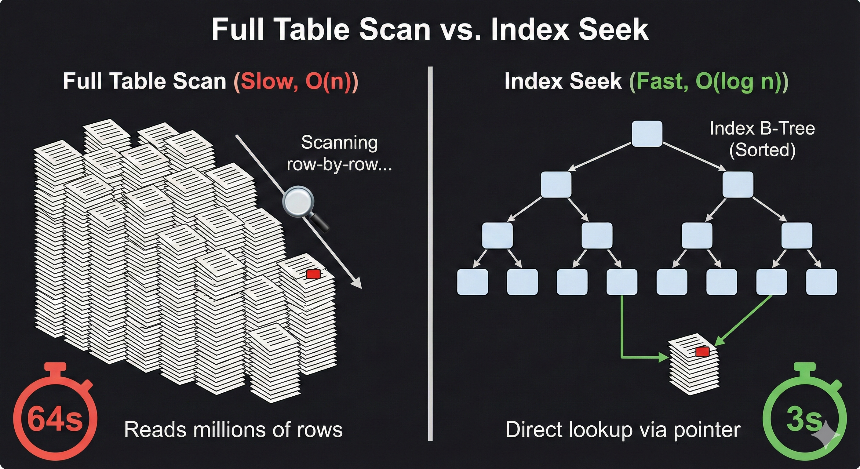
Binary Tree vs B-Tree
Binary Tree
50
/ \
30 70
/ \ / \
20 40 60 80
- Max 2 children per node
- Used in memory structures
- Can become unbalanced
- Height grows quickly
- Good for CPU operations
B-Tree
[30 | 60]
/ | \
[10 20] [40 50] [70 80 90]
- Many children per node
- Optimized for disk storage
- Always balanced
- Shallow height
- Used in database indexes
B-Tree Shape
- Many keys per node (high fanout)
- Height remains small
- Short height means few page reads
- Supports ordered traversal
[ 5000 | 9000 ]
/ | \
[1000|3000] [6000|7000] [10000|15000]
/ \ | / \
... ... ... ... ...
Index Example
CREATE INDEX idx_price
ON flowers(price);
- B-Tree is default index type
- Speeds up WHERE price = ...
- Speeds up ORDER BY price
- Used in SQLite, MariaDB, PostgreSQL
Why Shallow B-Trees Are Faster
Deep Binary Tree
Level 1 [50]
Level 2 [30] [70]
Level 3 [20] [40] [60] [80]
Level 4 ...
Level 5 ...
- Few keys per node
- Many levels
- Each level = disk page read
- More I/O operations
Shallow B-Tree
Level 1 [30 | 60 | 90]
Level 2 [10 20] [40 50] [70 80] [100 110]
- Many keys per node (high fanout)
- Very few levels
- Fewer disk page reads
- Optimized for storage systems
Example:
Fanout ≈ 1000
Level 1 → 1 node
Level 2 → 1000 nodes
Level 3 → 1,000,000 entries
Only 3 page reads to reach any row.
- Disk access is slower than memory
- Each level traversal = 1 page read
- Fewer levels = lower latency
- High fanout keeps tree shallow
B-Tree Split When Fanout Is Reached
- Each node has a maximum key capacity
- Fanout = maximum number of children
- If keys exceed capacity → node splits
- Middle key moves up to parent
- Tree remains balanced
Assume max 3 keys per node
Before insert:
[ 10 | 20 | 30 ]
Insert 40 → overflow:
[ 10 | 20 | 30 | 40 ]
After Split
[30]
/ \
[10 | 20] [40]
- Node divided into two
- Middle key promoted
- If parent is full → split propagates
- If root splits → height increases by 1
Index Fanout and Height
- Each node stores many keys per page
- High fanout → short tree height
- Short height → fewer page reads
- Main reason B-Trees scale on disk
High fanout example:
Level 1: [ 5000 | 9000 ]
/ | \
Level 2: [1000|3000] [6000|7000] [10000|15000]
/ \ | / \
Level 3: ... ... ... ... ...
More keys per node → Fewer levels
Fewer levels → Fewer page reads
Why It Matters
- Disk I/O is slower than memory
- Each level = one page read
- High fanout keeps tree shallow
- Shallow tree improves lookup speed
Height 3 tree:
Root → Internal → Leaf
= 3 page reads
Height 6 tree:
= 6 page reads
Create Index for User Lookups
- Builds a B-Tree on
user_id - Speeds up user-based lookups
- Improves search from O(n) → O(log n)
- Confirm usage with
EXPLAIN
CREATE INDEX idx_posts_user
ON posts(user_id);
Example Query
SELECT *
FROM posts
WHERE user_id = 42;
- Without index → full table scan
- With index → direct B-Tree lookup
- Index stores sorted keys
- Leaf nodes point to matching rows
Index for Time Ranges
- Jump to first key in range (O(log n))
- Scan forward in sorted order
- Stop when range condition fails
- Efficient for recent-post queries
CREATE INDEX idx_posts_created
ON posts(created_at);
Example Range Query
SELECT *
FROM posts
WHERE created_at >= '2026-01-01'
AND created_at < '2026-02-01'
ORDER BY created_at;
- B-Tree jumps to 2026-01-01
- Reads forward sequentially
- Stops after 2026-01-31
- No full table scan
Composite Index for Filter and Order
- Filter by
user_idand order bycreated_at - Reduces sorting work
- Works best with
LIMIT - Matches common feed patterns
CREATE INDEX idx_user_created
ON posts(user_id, created_at);
Example Query
SELECT *
FROM posts
WHERE user_id = 42
ORDER BY created_at DESC
LIMIT 10;
- Index first filters by
user_id - Rows already ordered by
created_at - No extra sort step needed
- Efficient for user feeds
Using LIMIT with Index
- Feeds often request “top 20” posts
- With a suitable index, engine can stop early
- Less scanning, faster response
- Works well with composite indexes
SELECT post_id, created_at
FROM posts
WHERE user_id = 5001
ORDER BY created_at DESC
LIMIT 20;Predicate Types and Index Use
| Predicate | Index Friendly? | Reason |
|---|---|---|
= |
Yes | Exact match |
BETWEEN |
Yes | Range scan |
LIKE 'abc%' |
Often | Prefix search |
LIKE '%abc' |
No | Leading wildcard breaks ordering |
Good: user_id = 5001
Good: created_at BETWEEN a AND b
Bad: content LIKE '%hello%'Indexing TEXT Content
contentis TEXT (large)- B-Tree is not ideal for substring search
- Can create large indexes and slow writes
- Keep B-Tree indexes for filters/sorts
- Use full-text search (separate topic)
- Or an external search engine
SHOW INDEX (MariaDB Introspection)
- Verify which indexes exist
- See key columns and sequence
- Check uniqueness and cardinality
- Review for redundancy
SHOW INDEX FROM posts;ANALYZE TABLE (Statistics Refresh)
- Optimizer relies on statistics
- Bad stats can lead to poor plan selection
- Refresh after large data changes
ANALYZE TABLE posts;Improves cardinality estimates used by the optimizer.
Indexing Is a Process
- At table creation time, query often incomplete
- Data volumes and user behavior change over time
- Indexes should be refined using evidence
- Continuous improvement keeps performance stable
- Workflow
- Observe queries
- Analyze plans
- Adjust indexes
Uncertainty at Design Time
| At Design Time | After Deployment | Consequence |
|---|---|---|
| Assumed common filters | Different filters dominate | Need new indexes |
| Estimated row counts | Data grows faster than expected | Scans become too slow |
| Simple queries expected | Composite patterns appear | Need composite indexes |
Measure and Verify (MariaDB)
- Use
EXPLAINto see plan choices - Confirm index usage and estimated rows
- Re-check after schema/index changes
- Refresh stats if estimates drift
EXPLAIN
SELECT *
FROM posts
WHERE user_id = 5001;Risks of Indexing
- Indexes consume disk space
- More memory pressure for caching
- More objects to maintain and monitor
- Too many indexes can complicate tuning
- Trade-off
- Over-indexing slows writes
- Under-indexing slows reads
- Choose based on measured workload
Heavy Write Tables: Trade-Off
| Write Pattern | What indexes add | Risk |
|---|---|---|
| Frequent INSERT | Each index must be updated | Throughput drops |
| UPDATE of indexed column | Reposition key in B-Tree | Higher write cost |
| Bulk ingestion | Many index page writes | Long ingest times |
Maintenance Cost (Complexity View)
| Operation | Cost with 0 extra indexes | Cost with k indexes |
|---|---|---|
| INSERT | Lower overhead | O(k · log n) |
| UPDATE indexed column | Lower overhead | O(k · log n) |
| DELETE | Lower overhead | O(k · log n) |
Balanced Strategy
- Start with minimal indexes tied to primary use cases
- Add composite indexes only for repeated patterns
- Avoid indexing low-selectivity columns alone
- Remove unused indexes over time
- Operational practice
- Measure latency and plans
- Adjust indexes
- Re-measure after changes
MariaDB Demo – Populate 500,000 Rows
1️⃣ Create Table
CREATE TABLE posts (
id INT AUTO_INCREMENT PRIMARY KEY,
user_id INT,
created_at DATETIME,
content VARCHAR(100)
);
2️⃣ Insert 500,000 Rows
WITH RECURSIVE seq AS (
SELECT 1 AS n
UNION ALL
SELECT n + 1 FROM seq WHERE n < 500000
)
INSERT INTO posts (user_id, created_at, content)
SELECT
FLOOR(RAND()*10000),
NOW() - INTERVAL FLOOR(RAND()*365) DAY,
CONCAT('Post ', n)
FROM seq;
- Generates 500k synthetic posts
- Random user_id (0–9999)
- Random date within last year
- Simulates production-like dataset
- Enough rows to observe index impact
MariaDB Demo – Populate 500,000 Rows (Compatible)
1️⃣ Create Table
DROP TABLE IF EXISTS posts;
CREATE TABLE posts (
id INT AUTO_INCREMENT PRIMARY KEY,
user_id INT NOT NULL,
created_at DATETIME NOT NULL,
content VARCHAR(100) NOT NULL
);
2️⃣ Insert 500,000 Rows (Numbers via CROSS JOIN)
INSERT INTO posts (user_id, created_at, content)
SELECT
FLOOR(RAND() * 10000) AS user_id,
NOW() - INTERVAL FLOOR(RAND() * 365) DAY AS created_at,
CONCAT('Post ', n) AS content
FROM (
SELECT
(a.d + 10*b.d + 100*c.d + 1000*d.d + 10000*e.d) + 1 AS n
FROM (SELECT 0 d UNION ALL SELECT 1 UNION ALL SELECT 2 UNION ALL SELECT 3 UNION ALL SELECT 4
UNION ALL SELECT 5 UNION ALL SELECT 6 UNION ALL SELECT 7 UNION ALL SELECT 8 UNION ALL SELECT 9) a
CROSS JOIN (SELECT 0 d UNION ALL SELECT 1 UNION ALL SELECT 2 UNION ALL SELECT 3 UNION ALL SELECT 4
UNION ALL SELECT 5 UNION ALL SELECT 6 UNION ALL SELECT 7 UNION ALL SELECT 8 UNION ALL SELECT 9) b
CROSS JOIN (SELECT 0 d UNION ALL SELECT 1 UNION ALL SELECT 2 UNION ALL SELECT 3 UNION ALL SELECT 4
UNION ALL SELECT 5 UNION ALL SELECT 6 UNION ALL SELECT 7 UNION ALL SELECT 8 UNION ALL SELECT 9) c
CROSS JOIN (SELECT 0 d UNION ALL SELECT 1 UNION ALL SELECT 2 UNION ALL SELECT 3 UNION ALL SELECT 4
UNION ALL SELECT 5 UNION ALL SELECT 6 UNION ALL SELECT 7 UNION ALL SELECT 8 UNION ALL SELECT 9) d
CROSS JOIN (SELECT 0 d UNION ALL SELECT 1 UNION ALL SELECT 2 UNION ALL SELECT 3 UNION ALL SELECT 4) e
) nums
WHERE n <= 500000;
- Generates integers 1..500000
- No CTE required
- Works on older MariaDB
- Random user_id and timestamps
SELECT COUNT(*) FROM posts;
Query Performance – With vs Without Index
Without Index
EXPLAIN ANALYZE
SELECT *
FROM posts
WHERE user_id = 500
ORDER BY created_at DESC
LIMIT 20;
- Full table scan
- Filesort required
- O(n)
Add Composite Index
CREATE INDEX idx_user_created
ON posts(user_id, created_at DESC);
With Index
EXPLAIN ANALYZE
SELECT *
FROM posts
WHERE user_id = 500
ORDER BY created_at DESC
LIMIT 20;
- Index range scan
- No filesort
- Stops after 20 rows
- O(log n)
Today
- Indexing in MariaDB
- Indexing in SQLite
- Indexing in PostgreSQL
- Compare systems
- Todo App: task table
- Insert 10,000 rows
- Performance before/after indexing
- Two-column index + sorting

What Is an Index?

Scan vs Index
- Database checks rows one-by-one
- Work grows with table size
- Time complexity: O(n)
- Database navigates the tree
- Jumps close to the target
- Time complexity: O(log n)

MariaDB Indexing (InnoDB)
- Primary key = clustered index
- Secondary indexes = B-Tree
- Composite indexes supported (multiple columns)
- Good introspection:
SHOW INDEX,EXPLAIN
SHOW INDEX FROM tasks;
EXPLAIN SELECT * FROM tasks WHERE status='done';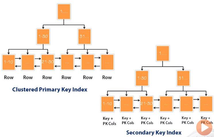
B-Tree vs Clustered Index: Similarities
- Both use a B-Tree structure
- Both keep keys sorted
- Both reduce search from O(n) → O(log n)
- Both improve read performance
-- Todo example
CREATE INDEX idx_status
ON tasks(status);
Whether clustered or not, the internal structure is still a B-Tree.
- B-Tree = the structure (how it works)
- Clustered = how the data is stored
B-Tree vs Clustered Index: Differences
| Aspect | B-Tree Index | Clustered Index |
|---|---|---|
| What is sorted? | Only the index | The actual table rows |
| How many allowed? | Many | Only one |
| Example | idx_status |
PRIMARY KEY (id) |
| Data storage | Separate from table | Data stored in that order |
- If PK = id → rows stored in id order
- If you create index on status → only the index is sorted
- Data rows stay in primary key order
Clustered / Primary-Key Index Support (MariaDB vs SQLite vs PostgreSQL)
| Database | Is PRIMARY KEY auto-indexed? | Are rows stored in PK order (clustered)? | Beginner takeaway |
|---|---|---|---|
| MariaDB (InnoDB) | Yes (auto B-Tree) | Yes (clustered by PK) | Table data “lives” in the PK B-Tree |
| SQLite | Yes (practically, via rowid / PK) | Often yes (rowid order is the storage order) | Rowid acts like the built-in key ordering |
| PostgreSQL | Yes (auto B-Tree) | No (heap table, not clustered by default) | PK index exists, but rows are stored separately |
- Auto-indexed PK means: DB creates an index for the PK.
- Clustered means: the table rows are physically stored in the index order.
CREATE TABLE tasks (
id INT PRIMARY KEY,
title VARCHAR(100),
status VARCHAR(20),
created_at DATETIME
);- InnoDB: rows stored by
id - SQLite: rows stored by rowid/PK
- Postgres: rows stored in heap, PK index separate
Why Clustered Storage Matters
- Rows are stored in PRIMARY KEY order
- Range queries become faster
- Sequential reads are efficient
- Less random disk access
SELECT *
FROM tasks
WHERE id BETWEEN 100 AND 200;
- InnoDB reads rows sequentially
- Rows are physically next to each other
- Index finds matching IDs
- Then fetches rows from heap
- May require more random reads
Questions?
SQLite Indexing
- Embedded DB (single file)
- B-Tree for tables and indexes
- Rowid tables by default
- Great for local apps, prototypes, small services
EXPLAIN QUERY PLAN
SELECT * FROM tasks WHERE status='done';PostgreSQL Indexing
- Default index: B-Tree
- Also supports: Hash, GIN, GiST, BRIN
- Strong planner (cost-based)
- Use:
EXPLAIN (ANALYZE, BUFFERS)
EXPLAIN (ANALYZE, BUFFERS)
SELECT * FROM tasks WHERE status='done';Comparison: MariaDB vs SQLite vs PostgreSQL
| Feature | MariaDB | SQLite | PostgreSQL |
|---|---|---|---|
| Default index | B-Tree | B-Tree | B-Tree |
| Runs as | Server | Embedded | Server |
| Clustered PK | Yes (InnoDB) | Rowid behavior | No (heap table) |
| Advanced index types | Limited | Minimal | Many |
Todo App: Task Table
- We will query by
statusand sort bycreated_at - That workload is perfect to show index impact
-- Logical schema
id, title, status, priority, created_at
Create Table: MariaDB
DROP TABLE IF EXISTS tasks;
CREATE TABLE tasks (
id INT AUTO_INCREMENT PRIMARY KEY,
title VARCHAR(255) NOT NULL,
status VARCHAR(20) NOT NULL,
priority INT NOT NULL,
created_at DATETIME NOT NULL
) ENGINE=InnoDB;Create Table: SQLite + PostgreSQL
-- SQLite
CREATE TABLE tasks (
id INTEGER PRIMARY KEY,
title TEXT NOT NULL,
status TEXT NOT NULL,
priority INTEGER NOT NULL,
created_at TEXT NOT NULL
);
-- PostgreSQL
CREATE TABLE tasks (
id SERIAL PRIMARY KEY,
title VARCHAR(255) NOT NULL,
status VARCHAR(20) NOT NULL,
priority INT NOT NULL,
created_at TIMESTAMP NOT NULL
);Insert 10,000 Rows (MariaDB Demo)
INSERT INTO tasks (title, status, priority, created_at)
SELECT
CONCAT('Task ', n),
ELT(FLOOR(1 + RAND()*3),'open','in_progress','done'),
FLOOR(RAND()*5),
NOW() - INTERVAL FLOOR(RAND()*30) DAY
FROM (
SELECT (a.d + 10*b.d + 100*c.d + 1000*d.d) + 1 AS n
FROM (SELECT 0 d UNION ALL SELECT 1 UNION ALL SELECT 2 UNION ALL SELECT 3 UNION ALL SELECT 4
UNION ALL SELECT 5 UNION ALL SELECT 6 UNION ALL SELECT 7 UNION ALL SELECT 8 UNION ALL SELECT 9) a
CROSS JOIN (SELECT 0 d UNION ALL SELECT 1 UNION ALL SELECT 2 UNION ALL SELECT 3 UNION ALL SELECT 4
UNION ALL SELECT 5 UNION ALL SELECT 6 UNION ALL SELECT 7 UNION ALL SELECT 8 UNION ALL SELECT 9) b
CROSS JOIN (SELECT 0 d UNION ALL SELECT 1 UNION ALL SELECT 2 UNION ALL SELECT 3 UNION ALL SELECT 4
UNION ALL SELECT 5 UNION ALL SELECT 6 UNION ALL SELECT 7 UNION ALL SELECT 8 UNION ALL SELECT 9) c
CROSS JOIN (SELECT 0 d UNION ALL SELECT 1 UNION ALL SELECT 2 UNION ALL SELECT 3 UNION ALL SELECT 4
UNION ALL SELECT 5 UNION ALL SELECT 6 UNION ALL SELECT 7 UNION ALL SELECT 8 UNION ALL SELECT 9) d
) nums
WHERE n <= 10000;
SELECT COUNT(*) FROM tasks;Insert 10,000 Rows (SQLite)
WITH RECURSIVE seq(n) AS (
SELECT 1
UNION ALL
SELECT n + 1 FROM seq WHERE n < 10000
)
INSERT INTO tasks (title, status, priority, created_at)
SELECT
'Task ' || n,
CASE (ABS(RANDOM()) % 3)
WHEN 0 THEN 'open'
WHEN 1 THEN 'in_progress'
ELSE 'done'
END,
ABS(RANDOM()) % 5,
DATETIME('now', '-' || (ABS(RANDOM()) % 30) || ' days')
FROM seq;
SELECT COUNT(*) FROM tasks;
Insert 10,000 Rows (PostgreSQL)
INSERT INTO tasks (title, status, priority, created_at)
SELECT
'Task ' || n,
(ARRAY['open','in_progress','done'])[floor(random()*3)+1],
floor(random()*5),
NOW() - (floor(random()*30) || ' days')::interval
FROM generate_series(1,10000) AS n;
SELECT COUNT(*) FROM tasks;
Workload Query #1: Filter by status (Before Index) — All 3 Databases
SELECT *
FROM tasks
WHERE status = 'done';- Before indexing, the DB often scans many rows to find
status='done' - We use each DB’s “plan/explain” tool to confirm what it does
| DB | Plan / Analyzer Command |
|---|---|
| MariaDB |
|
| PostgreSQL |
|
| SQLite |
|
Add Single-Column Index (status)
CREATE INDEX idx_tasks_status
ON tasks(status);CREATE INDEX idx_tasks_status
ON tasks(status);CREATE INDEX idx_tasks_status
ON tasks(status);- Same SQL syntax across all three systems
- Creates a B-Tree index by default
- Speeds up:
WHERE status = 'done' - Keys are stored sorted by
status - Reduces scan from O(n) → O(log n)
- Does not change table row order
- Only affects lookup speed
Workload Query #1: After Index — Analyze (All 3 Databases)
EXPLAIN
SELECT *
FROM tasks
WHERE status = 'done';EXPLAIN ANALYZE
SELECT *
FROM tasks
WHERE status = 'done';EXPLAIN QUERY PLAN
SELECT *
FROM tasks
WHERE status = 'done';- After creating
idx_tasks_status - Planner should show index usage
- MariaDB: type = ref / key used
- Postgres: Index Scan
- SQLite: SEARCH TABLE using index
- Full table scan should disappear
- Root → Internal → Leaf
- Direct lookup replaces scanning
Workload Query #2: Sort by created_at (Before Composite Index)
EXPLAIN ANALYZE
SELECT *
FROM tasks
WHERE status = 'done'
ORDER BY created_at DESC
LIMIT 20;- If only
idx_tasks_statusexists, DB may still need to sort - Sorting can be expensive (extra work + memory + temp files)
Why Two-Column Index Helps Sorting
(status, created_at)
- Index is sorted first by
status - Within each status, it is sorted by
created_at - So the DB can read rows already in the right order
-- Think: ordered groups
(status='done', newest → oldest)
(status='open', newest → oldest)
(status='in_progress', newest → oldest)Two-Index Keys: Concrete Mini Example
| status | created_at | title |
|---|---|---|
| done | 2026-02-25 10:05 | Task A |
| open | 2026-02-25 09:00 | Task B |
| done | 2026-02-25 08:10 | Task C |
| done | 2026-02-24 20:00 | Task D |
- All
donerows are next to each other - Already ordered newest → oldest
LIMIT 20can stop early (fast)
Create Composite Index for Filter + Sort
-- MariaDB
CREATE INDEX idx_status_created
ON tasks(status, created_at DESC);
-- SQLite (DESC allowed in index; planner may still optimize)
CREATE INDEX idx_status_created
ON tasks(status, created_at);
-- PostgreSQL
CREATE INDEX idx_status_created
ON tasks(status, created_at DESC);- This index matches:
WHERE status=? ORDER BY created_at DESC - Reduces or removes the sort step
Query After Composite Index (Expected Improvement)
EXPLAIN ANALYZE
SELECT *
FROM tasks
WHERE status = 'done'
ORDER BY created_at DESC
LIMIT 20;- Planner can do an index range scan
- No big sort needed
- Reads only the first 20 matching rows
Questions?
Today
- Indexing in MariaDB
- Review Homework 2
- Review Lab 2
- Midterm (next Friday)
What Is an Index?
MariaDB Indexing (InnoDB)
- Primary key = clustered index
- Secondary indexes = B-Tree
- Composite indexes supported (multiple columns)
- Good introspection:
SHOW INDEX,EXPLAIN
SHOW INDEX FROM tasks;
EXPLAIN SELECT * FROM tasks WHERE status='done';Why Clustered Storage Matters
- Rows are stored in PRIMARY KEY order
- Range queries become faster
- Sequential reads are efficient
- Less random disk access
SELECT *
FROM tasks
WHERE id BETWEEN 100 AND 200;
- InnoDB reads rows sequentially
- Rows are physically next to each other
- Index finds matching IDs
- Then fetches rows from heap
- May require more random reads
Questions?
Todo App: Task Table
- We will query by
statusand sort bycreated_at - That workload is perfect to show index impact
-- Logical schema
id, title, status, priority, created_atCreate Table: MariaDB
DROP TABLE IF EXISTS tasks;
CREATE TABLE tasks (
id INT AUTO_INCREMENT PRIMARY KEY,
title VARCHAR(255) NOT NULL,
status VARCHAR(20) NOT NULL,
priority INT NOT NULL,
created_at DATETIME NOT NULL
) ENGINE=InnoDB;Insert 10,000 Rows (MariaDB Demo)
INSERT INTO tasks (title, status, priority, created_at)
SELECT
CONCAT('Task ', n),
ELT(FLOOR(1 + RAND()*3),'open','in_progress','done'),
FLOOR(RAND()*5),
NOW() - INTERVAL FLOOR(RAND()*30) DAY
FROM (
SELECT (a.d + 10*b.d + 100*c.d + 1000*d.d) + 1 AS n
FROM (SELECT 0 d UNION ALL SELECT 1 UNION ALL SELECT 2 UNION ALL SELECT 3 UNION ALL SELECT 4
UNION ALL SELECT 5 UNION ALL SELECT 6 UNION ALL SELECT 7 UNION ALL SELECT 8 UNION ALL SELECT 9) a
CROSS JOIN (SELECT 0 d UNION ALL SELECT 1 UNION ALL SELECT 2 UNION ALL SELECT 3 UNION ALL SELECT 4
UNION ALL SELECT 5 UNION ALL SELECT 6 UNION ALL SELECT 7 UNION ALL SELECT 8 UNION ALL SELECT 9) b
CROSS JOIN (SELECT 0 d UNION ALL SELECT 1 UNION ALL SELECT 2 UNION ALL SELECT 3 UNION ALL SELECT 4
UNION ALL SELECT 5 UNION ALL SELECT 6 UNION ALL SELECT 7 UNION ALL SELECT 8 UNION ALL SELECT 9) c
CROSS JOIN (SELECT 0 d UNION ALL SELECT 1 UNION ALL SELECT 2 UNION ALL SELECT 3 UNION ALL SELECT 4
UNION ALL SELECT 5 UNION ALL SELECT 6 UNION ALL SELECT 7 UNION ALL SELECT 8 UNION ALL SELECT 9) d
) nums
WHERE n <= 10000;
SELECT COUNT(*) FROM tasks;Workload Query #1: Filter by status (Before Index) — All 3 Databases
SELECT *
FROM tasks
WHERE status = 'done';- Before indexing, the DB often scans many rows to find
status='done' - We use each DB’s “plan/explain” tool to confirm what it does
| DB | Plan / Analyzer Command |
|---|---|
| MariaDB |
|
| PostgreSQL |
|
| SQLite |
|
Add Single-Column Index (status)
CREATE INDEX idx_tasks_status
ON tasks(status);CREATE INDEX idx_tasks_status
ON tasks(status);CREATE INDEX idx_tasks_status
ON tasks(status);- Same SQL syntax across all three systems
- Creates a B-Tree index by default
- Speeds up:
WHERE status = 'done' - Keys are stored sorted by
status - Reduces scan from O(n) → O(log n)
- Does not change table row order
- Only affects lookup speed
Workload Query #1: After Index — Analyze (All 3 Databases)
EXPLAIN
SELECT *
FROM tasks
WHERE status = 'done';EXPLAIN ANALYZE
SELECT *
FROM tasks
WHERE status = 'done';EXPLAIN QUERY PLAN
SELECT *
FROM tasks
WHERE status = 'done';- After creating
idx_tasks_status - Planner should show index usage
- MariaDB: type = ref / key used
- Postgres: Index Scan
- SQLite: SEARCH TABLE using index
- Full table scan should disappear
- Root → Internal → Leaf
- Direct lookup replaces scanning
Workload Query #2: Sort by created_at (Before Composite Index)
EXPLAIN ANALYZE
SELECT *
FROM tasks
WHERE status = 'done'
ORDER BY created_at DESC
LIMIT 20;- If only
idx_tasks_statusexists, DB may still need to sort - Sorting can be expensive (extra work + memory + temp files)
Why Two-Column Index Helps Sorting
(status, created_at)
- Index is sorted first by
status - Within each status, it is sorted by
created_at - So the DB can read rows already in the right order
-- Think: ordered groups
(status='done', newest → oldest)
(status='open', newest → oldest)
(status='in_progress', newest → oldest)Two-Index Keys: Concrete Mini Example
| status | created_at | title |
|---|---|---|
| done | 2026-02-25 10:05 | Task A |
| open | 2026-02-25 09:00 | Task B |
| done | 2026-02-25 08:10 | Task C |
| done | 2026-02-24 20:00 | Task D |
- All
donerows are next to each other - Already ordered newest → oldest
LIMIT 20can stop early (fast)
Create Composite Index for Filter + Sort
-- MariaDB
CREATE INDEX idx_status_created
ON tasks(status, created_at DESC);
-- SQLite (DESC allowed in index; planner may still optimize)
CREATE INDEX idx_status_created
ON tasks(status, created_at);
-- PostgreSQL
CREATE INDEX idx_status_created
ON tasks(status, created_at DESC);- This index matches:
WHERE status=? ORDER BY created_at DESC - Reduces or removes the sort step
Query After Composite Index (Expected Improvement)
EXPLAIN ANALYZE
SELECT *
FROM tasks
WHERE status = 'done'
ORDER BY created_at DESC
LIMIT 20;- Planner can do an index range scan
- No big sort needed
- Reads only the first 20 matching rows
Questions?
Why SQLite for Mobile Apps?
- Lightweight engine ideal for phones
- No setup required on iOS or Android
- Works fully offline inside the app
- Fast local storage for user data
- Reliable: used by thousands of mobile apps
- Free and built into both platforms

Embedded Database
- An embedded database runs inside an application
- No separate database server process
- Database engine is a library
- Data stored in a single file
Application
|
| SQLite library
|
flowers.db ← file on disk
- SQLite is embedded
- No network connection needed
- Ideal for local apps, tools, mobile
Single Process (Embedded SQLite)
Application Code
(Java · Python · C++ · JS)
│
│ SQLite library
│ parse · plan · execute
│
Database File
flowers.db
(tables · rows · indexes)
Where SQLite Is Installed by Default
SQLite is included out of the box on many devices and operating systems.
- iPhone / iOS: Core Data can store data in SQLite
- Android: Every device includes SQLite for app storage
- macOS: System utilities and Spotlight use SQLite
- Windows 10/11: Many system tools rely on SQLite
- Linux distributions: Included in most installations
- Smart TVs / Set-top boxes: Used for settings and logs
- Gaming consoles: Stores local game and device data
- IoT devices: Favored for low-memory environments
Chronology of SQLite Versions
- 2000 – Version 1.0: Basic SQL support
- 2001 – Version 2.0: Transactions added
- 2004 – Version 3.0: UTF-8, BLOBs, improved queries

Recent SQLite Updates (Example)
Fix typos in climode.html
- Update corrected spelling issues in CLI documentation.
- Small changes improve clarity for developers.
- SQLite team maintains quality careful refinement.

SQLite Licensing
Open Parts ✔️
- You may read the full source code
- You may download the code freely
- You may change or modify the code
- SQLite is in the public domain
- No royalties, no restrictions for commercial use
- GitHub: github.com/sqlite/sqlite
Closed or Protected Parts 🔒
- The official main branch is write protected
- Core maintainers may commit main repository
- Public contributions require review before merging
- No direct write access to SQLite’s Fossil repo
- Release process is controlled by core team
- Trademark usage (SQLite logos) has restrictions
ALTER TABLE: Supported in SQLite
-- rename a table
ALTER TABLE flowers
RENAME TO plants;
-- add a new column
ALTER TABLE flowers
ADD COLUMN origin TEXT;
-- rename a column
ALTER TABLE flowers
RENAME COLUMN price TO unit_price;
- Limited but safe operations
- No data rewrite needed
- Works directly on the file
ALTER TABLE: Not Supported
-- remove a column
ALTER TABLE flowers
DROP COLUMN color;
-- change column type
ALTER TABLE flowers
ALTER COLUMN price REAL;
-- add multiple columns
ALTER TABLE flowers
ADD COLUMN size TEXT,
ADD COLUMN stock INTEGER;
- Requires table rebuild
- Not part of SQLite ALTER TABLE
- Handled via create-copy-drop
Install SQLite
- SQLite Download Page
- Download SQLite Tools (Windows x64)
- Unzip the package
- Add the folder to your PATH
- SQLite Online Editor
SQLite Browser Admin Interface
DB Browser for SQLite offers a simple graphical interface to manage SQLite databases.
- Create, browse, and edit tables
- Run SQL queries interactively
- Import and export CSV, SQL, JSON
- View data without writing commands
- Works on Windows, macOS, and Linux
- https://sqlitebrowser.org

SQLite Workflow
- Create Database
- Create Table
- Insert Data
sqlite3 database_name.db
CREATE TABLE table_name (
column1 datatype,
column2 datatype
);
INSERT INTO table_name (column1, column2)
VALUES (value1, value2);
Executing SQL Commands
- From Python
import sqlite3
conn = sqlite3.connect("db.db")
cur = conn.cursor()
cur.execute("SELECT * FROM table_name;")
val db = SQLiteDatabase.openOrCreateDatabase("db.db", null)
val cursor = db.rawQuery("SELECT * FROM table_name;", null)
- From C++
#include "sqlite3.h"
sqlite3 *db;
sqlite3_open("db.db", &db);
sqlite3_exec(db, "SELECT * FROM table_name;", 0, 0, 0);
import SQLite3
var db: OpaquePointer?
sqlite3_open("db.db", &db)
sqlite3_exec(db, "SELECT * FROM table_name;", nil, nil, nil)
ACID in SQLite ✔️
ACID Basics
- All-or-nothing writes
- Consistent state after commits
- Snapshot isolation for readers
- Data stored safely on disk
Isolation
- Many readers allowed
- One writer at a time
Multi-User Limits ⚠️
- Not built for many writers
- Writes lock the whole DB
- High write load slows apps
- No client-server model
- Use server DBs for scale
SQLite and SQL Standards
- SQLite follows the traditional SQL syntax
- Most commands align with long-standing SQL practice
- Constraint enforcement is relaxed by default
- Foreign keys exist but are not enforced automatically
- Developers must turn enforcement on manually
- This behavior comes from SQLite’s embedded roots
PRAGMA foreign_keys = ON;
PRAGMA foreign_keys;
SQLite Dot Commands
- .databases – List all attached DBs
- .tables – Show tables
- .schema – Show schema
- .read – Execute script
- .exit – Leave shell
- .help – All commands
- documentation
Plant Watering App: Two Tables
Plant Table
CREATE TABLE Plant (
PlantID INTEGER PRIMARY KEY,
Name TEXT NOT NULL,
WaterThreshold FLOAT
);
SensorData Table
CREATE TABLE SensorData (
SensorDataID INTEGER PRIMARY KEY,
PlantID INTEGER NOT NULL,
WaterLevel FLOAT,
Timestamp DATETIME,
FOREIGN KEY (PlantID) REFERENCES Plant(PlantID)
);
CRUD Operations (Create + Read)
Create
INSERT INTO Plant (Name, WaterThreshold)
VALUES ('Aloe Vera', 30);
INSERT INTO SensorData (PlantID, WaterLevel, Timestamp)
VALUES (1, 22, '2025-11-27 10:00');
Read
SELECT *
FROM Plant;
SELECT PlantID, WaterLevel
FROM SensorData
ORDER BY Timestamp DESC;
CRUD Operations (Update + Delete)
Update
UPDATE Plant
SET WaterThreshold = 40
WHERE PlantID = 1;
UPDATE SensorData
SET WaterLevel = 18
WHERE SensorDataID = 1;
Delete
DELETE FROM Plant
WHERE PlantID = 3;
DELETE FROM SensorData
WHERE Timestamp < '2025-01-01';
SQLite CLI Commands and Pragmas
Dot Commands
- .database
- .table
- .schema
- .help
PRAGMA Settings
PRAGMA foreign_keys = ON;
PRAGMA foreign_keys;
Foreign Key Violation
INSERT INTO SensorData (PlantID, WaterLevel, Timestamp)
VALUES (999, 50, '2025-11-27 11:00');
SQLite Data Types: Declared vs Enforced
- VARCHAR(2)
- CHAR(5)
- TEXT NOT NULL
- BOOLEAN
- DATE / DATETIME
- Custom names (EMAIL, NAME, PHONE)
CREATE TABLE User (
Name VARCHAR(2)
);
- No length checking on VARCHAR
- VARCHAR(2) is stored as TEXT
- Strings of any length allowed
- BOOLEAN becomes INTEGER
- DATE stored as TEXT/REAL/INTEGER
- Only NULL, INTEGER, REAL, TEXT, BLOB enforced
INSERT INTO User (Name)
VALUES ('ABCDE'); -- Works!
-- Strict mode needed for real enforcement
CREATE TABLE UserStrict (
Name TEXT
) STRICT;
Useful SQLite Links
PostgreSQL
Chronological Timeline
- 1977 – INGRES project begins at UC Berkeley
- 1986 – POSTGRES research project starts
- 1994 – SQL support added to POSTGRES
- 1996 – Renamed to PostgreSQL
- Today – Global open source database
People
- POSTGRES = “POST INGRES”
- Built as the successor to INGRES
- Led by Michael Stonebraker
- Focused on extensibility and advanced data types
- PostgreSQL emphasizes SQL support
PostgreSQL Market Share
Relational Database Usage (Approx.)
- MySQL: ~35–40%
- PostgreSQL: ~15–20%
- SQL Server: ~15%
- Oracle DB: ~10%
- SQLite: Widely embedded (not server share)
Positioning
- Fastest growing open source relational DB
- Strong adoption in cloud and startups
- Preferred for advanced SQL and data integrity
- Common alternative to commercial databases
- Backed by long academic and open source lineage
PostgreSQL Links & Resources
Official & Community
- Official Website: https://www.postgresql.org/
- Documentation: https://www.postgresql.org/docs/
- GitHub: https://github.com/postgres/postgres
- Mailing Lists: https://www.postgresql.org/list/
Ecosystem & Tools
- pgAdmin: https://www.pgadmin.org/
- PostgreSQL Wiki: https://wiki.postgresql.org/
- Extensions: postgresql.org/.../contrib.html
PostgreSQL License
License Requirements
- Permissive open source license
- Free for commercial and private use
- Modification allowed
- Redistribution allowed
- Copyright notice must be included
- No warranty provided
License Text (Excerpt)
PostgreSQL Database Management System
(formerly known as Postgres, then Postgres95)
Copyright (c) 1996–2024,
The PostgreSQL Global Development Group
Permission to use, copy, modify, and distribute this
software and its documentation for any purpose, without
fee, and without a written agreement is hereby granted,
provided that the above copyright notice and this
paragraph appear in all copies.
IN NO EVENT SHALL THE POSTGRESQL GLOBAL DEVELOPMENT
GROUP BE LIABLE FOR ANY DAMAGES ARISING OUT OF THE
USE OF THIS SOFTWARE.
Why PostgreSQL?
- Open source, enterprise class relational database
- Strong correctness tradition: ACID + MVCC
- Built for concurrency and long running systems
- Extensible: custom types, functions, extensions
- Used in research, startups, and large institutions
- Fits well when data outgrows embedded storage

SQLite vs PostgreSQL: Query Comparison
- File based embedded database
- Simple setup, zero configuration
- Good for local apps and learning
- Client server database system
- Multi user, concurrent access
- Production grade workloads
CREATE TABLE
CREATE TABLE users (
id INTEGER PRIMARY KEY,
name TEXT NOT NULL,
email TEXT UNIQUE
);
- INTEGER PRIMARY KEY auto increments
- Types are flexible
CREATE TABLE users (
id SERIAL PRIMARY KEY,
name VARCHAR(100) NOT NULL,
email VARCHAR(255) UNIQUE
);
- Explicit data types
- SERIAL generates sequence
INTEGER
product_id INTEGER
-- example: 101
- Type affinity
- INTEGER PRIMARY KEY auto increments
product_id INTEGER
-- example: 101
- Strict integer
- Common for primary keys
VARCHAR
product_name VARCHAR(100)
-- example: 'Oak Dining Table'
- Length not enforced
- Treated like TEXT
product_name VARCHAR(100)
-- example: 'Oak Dining Table'
- Length enforced
- Schema level constraint
TEXT
description TEXT
-- example: 'Solid wood table with natural finish'
- Unlimited length
- Flexible storage
description TEXT
-- example: 'Solid wood table with natural finish'
- Unlimited length
- Explicit text type
BOOLEAN
in_stock BOOLEAN
-- example: 1
- Stored as 0 or 1
- No strict enforcement
in_stock BOOLEAN
-- example: true
- true / false only
- Strict validation
DATE
release_date DATE
-- example: '2025-03-01'
- Stored as TEXT/INTEGER
- No engine validation
release_date DATE
-- example: '2025-03-01'
- Calendar date
- Validated by database
SERIAL vs AUTOINCREMENT
product_id INTEGER
PRIMARY KEY AUTOINCREMENT
-- example values: 1, 2, 3
- SQLite keyword
- Uses internal rowid
- Prevents reuse of deleted ids
product_id SERIAL PRIMARY KEY
-- example values: 1, 2, 3
- INTEGER + sequence
- Sequence is independent object
- Supports concurrent inserts
CHECK Constraints
price NUMERIC CHECK (price > 0)
-- example: 1299.99
- Supported but limited
- Evaluated at insert/update
price NUMERIC(10,2)
CHECK (price > 0 AND price < 20000)
-- example: 1299.99
- Fully enforced
- Complex expressions allowed
Date Functions
SELECT date('now');
-- example result: '2026-02-04'
SELECT date('now','+7 days');
-- example result: '2026-02-11'
- String based functions
- Limited set of modifiers
SELECT CURRENT_DATE;
-- example result: 2026-02-04
SELECT CURRENT_DATE + INTERVAL '7 days';
-- example result: 2026-02-11
- Rich date arithmetic
- Interval type supported
TIMESTAMP
created_at TIMESTAMP
-- example: '2025-03-01 10:30:00'
- Stored as string or number
- No timezone awareness
created_at TIMESTAMP
-- example: '2025-03-01 10:30:00'
- Date and time
- Rich date functions
TIMESTAMP WITH TIME ZONE
created_at TIMESTAMP
-- example: '2025-03-01 10:30:00'
- Timezone handled by application
- No UTC normalization
created_at TIMESTAMPTZ
-- example: '2025-03-01 18:30:00+00'
- Stored in UTC
- Session timezone aware
REAL
weight REAL
-- example: 45.5
- Floating point
- No precision guarantees
weight REAL
-- example: 45.5
- Floating point
- IEEE compliant
NUMERIC
price NUMERIC
-- example: 1299.99
- Flexible precision
- Not strictly enforced
price NUMERIC(10,2)
-- example: 1299.99
- Exact precision
- Best for money
JSON
specs JSON
-- example: '{"material":"oak","seats":6}'
- Stored as TEXT
- Limited querying
specs JSONB
-- example: '{"material":"oak","seats":6}'
- Binary JSON
- Indexable and queryable
PostgreSQL Attribute Data Types (Not in SQLite)
-- ENUM
status ENUM('draft','active','discontinued')
-- example: 'active'
-- ARRAY
tags TEXT[]
-- example: {'wood','dining','premium'}
-- JSONB
specs JSONB
-- example: {"material":"oak","seats":6}
-- UUID
product_uuid UUID
-- example: '550e8400-e29b-41d4-a716-446655440000'
-- INTERVAL
warranty INTERVAL
-- example: '2 years 6 months'
- ENUM: controlled values at schema level
- ARRAY: first-class multi-value columns
- JSONB: binary JSON with indexing and operators
- UUID: globally unique identifiers
- INTERVAL: native duration type for time math
- SQLite has no native support for these types
Querying PostgreSQL-Specific Data Types
-- ENUM
SELECT * FROM products WHERE status = 'active';
-- ARRAY
SELECT * FROM products WHERE 'wood' = ANY(tags);
-- JSONB
SELECT * FROM products WHERE specs->>'material' = 'oak';
-- UUID
SELECT *
FROM products
WHERE product_uuid = '550e8400-e29b-41d4-a716-446655440000';
-- INTERVAL
SELECT * FROM products WHERE warranty > INTERVAL '2 years';
- ENUM compared like strings, validated by schema
- ARRAY supports membership queries (ANY, ALL)
- JSONB supports key access and indexing
- UUID compared directly, no casting needed
- INTERVAL works in native time arithmetic
INSERT
INSERT INTO users (name, email)
VALUES ('Alice', 'alice@example.com');
- No RETURNING support (older versions)
- Last ID fetched separately
INSERT INTO users (name, email)
VALUES ('Alice', 'alice@example.com')
RETURNING id;
- RETURNING is built in
- Common in APIs
READ (SELECT)
SELECT id, name, email
FROM users
WHERE name = 'Alice';
- Simple query engine
- Single writer at a time
SELECT id, name, email
FROM users
WHERE name = 'Alice';
- Advanced optimizer
- Concurrent reads and writes
UPDATE
UPDATE users
SET email = 'new@example.com'
WHERE id = 1;
- No RETURNING clause
UPDATE users
SET email = 'new@example.com'
WHERE id = 1
RETURNING *;
- Can return updated rows
DELETE
DELETE FROM users
WHERE id = 1;
- Deletes row immediately
DELETE FROM users
WHERE id = 1
RETURNING id;
- Supports auditing patterns
TRANSACTIONS
BEGIN;
UPDATE users SET name = 'Bob';
COMMIT;
- Database level lock on write
BEGIN;
UPDATE users SET name = 'Bob';
COMMIT;
- MVCC allows concurrency
CONSTRAINTS
CREATE TABLE orders (
id INTEGER PRIMARY KEY,
user_id INTEGER,
FOREIGN KEY (user_id)
REFERENCES users(id)
);
- Foreign keys must be enabled
CREATE TABLE orders (
id SERIAL PRIMARY KEY,
user_id INT REFERENCES users(id)
);
- Constraints always enforced
DATA TYPES
- Dynamic typing
- TEXT, INTEGER, REAL
- Type affinity model
price TEXT
price INTEGER
price REAL
- Strong typing
- Numeric, JSON, UUID, arrays
price NUMERIC(10,2)
data JSONB
id UUID
When to Use Which
- Local apps
- Single user tools
- Teaching and prototyping
- Low operational overhead
- Multi user systems
- Concurrent workloads
- APIs and web apps
- Production systems
Client Server Database
- A server database runs as a separate service
- Multiple apps connect over the network
- Access controlled with roles and permissions
- Better for many users and concurrent writes
Application (Frontend / Backend)
|
| network connection (TCP)
|
PostgreSQL Server
| parse · plan · execute
|
Database Storage
(tables · rows · indexes)
- PostgreSQL is client server
- Designed for multi user workloads
- Central place for governance and auditing
Two Process View (Typical Deployment)
Client App
(Python · Java · Node · Go)
│
│ driver / protocol
│ authenticate · send SQL
▼
PostgreSQL Server
parse · plan · execute
│
▼
Storage
tables · rows · indexes
PostgreSQL: A Timeline
- 1986: Developed at UC Berkeley by Michael Stonebraker
- 1989: POSTGRES 1.0 released
- 1994: Renamed to PostgreSQL
- 1996: Open source development begins
- 2000: MVCC introduced in PostgreSQL 7.0
- 2005: Native Windows support added
- 2010: Streaming replication introduced
- 2016: Logical replication and partitioning added
- 2020: Improved indexing and query performance
- 2023: PostgreSQL 16 improves parallelism and SQL features
Why Was PostgreSQL Invented?
- Ingres limitations: needed extensibility and richer types
- Advanced data needs: better handling of objects and relationships
- Scalability: more flexible and efficient query engine
- ACID compliance: improved reliability and consistency
- Open source model: community contributions and long term continuity
SQLite vs PostgreSQL: Licensing
SQLite
- Public Domain
- No restrictions
- Free for any use
PostgreSQL
- PostgreSQL License (BSD style)
- Keep copyright notice
- Permissive for commercial use
PostgreSQL: Open Source License Requirements
| Database | License | Restrictions |
|---|---|---|
| SQLite | Public Domain | No restrictions, free for any use |
| PostgreSQL | PostgreSQL License (BSD style) | Requires keeping copyright notice |
PostgreSQL License Notice
PostgreSQL Database Management System
Copyright (c) 1996-2024, The PostgreSQL Global Development Group
Permission to use, copy, modify, and distribute this software and its
documentation for any purpose, without fee, and without a written
agreement is hereby granted, provided that the above copyright notice
and this paragraph appear in all copies.
IN NO EVENT SHALL THE AUTHORS OR COPYRIGHT HOLDERS BE LIABLE FOR ANY
CLAIM, DAMAGES, OR OTHER LIABILITY, WHETHER IN AN ACTION OF CONTRACT,
TORT OR OTHERWISE, ARISING FROM, OUT OF, OR IN CONNECTION WITH THE
SOFTWARE OR THE USE OR OTHER DEALINGS IN THE SOFTWARE.
PostgreSQL Feature Matrix
- SQL features and standards coverage
- Concurrency and replication options
- Index types and extensions
- Security and authentication methods
PostgreSQL Query Transformer
- SQL is parsed into an internal representation
- Rewrite and analysis happen before planning
- Planner chooses a physical execution plan
- This is where correctness meets efficiency
Relational Database Admin Interfaces
Neon Database Admin Functions
- Database management – create, delete, manage databases
- Branching – create database branches for development and testing
- Connection monitoring – active connections and resource usage
- Role and access control – manage users, roles, permissions
- Performance insights – analyze queries and execution cost
Neon Database Console
- Admin UI for hosted PostgreSQL
- Useful for quick setup and inspection
pg_stat_statements
- Tracks execution statistics of SQL queries
- Records query text, execution time, and I/O stats
- Helps identify slow or expensive queries
- Requires the
pg_stat_statementsextension - Useful for performance tuning and workload visibility
-- typical enable (often via postgresql.conf)
-- shared_preload_libraries = 'pg_stat_statements'
CREATE EXTENSION IF NOT EXISTS pg_stat_statements;
SELECT query, calls, total_exec_time
FROM pg_stat_statements
ORDER BY total_exec_time DESC
LIMIT 5;
UUID in PostgreSQL
- UUID = Universally Unique Identifier
- 128-bit globally unique value
- Safe for distributed systems
- No central sequence required
- Common in APIs and microservices
CREATE TABLE users (
id UUID PRIMARY KEY,
name TEXT
);
-- example value
'550e8400-e29b-41d4-a716-446655440000'
Generating UUID
- Requires extension
- Most common: pgcrypto
- UUID generated inside database
- Removes dependency on application logic
CREATE EXTENSION IF NOT EXISTS pgcrypto;
CREATE TABLE orders (
id UUID PRIMARY KEY DEFAULT gen_random_uuid(),
total NUMERIC(10,2)
);
INSERT INTO orders (total)
VALUES (99.99)
RETURNING id;
UUID vs SERIAL
id SERIAL PRIMARY KEY
-- 1,2,3,4
- Sequential
- Predictable
- Centralized sequence
id UUID PRIMARY KEY
-- random pattern
- Non predictable
- Safe for replication
- Good for public APIs
ARRAY Type
- PostgreSQL supports native arrays
- Single column can store multiple values
- Useful for tags, labels, categories
- First class type, not string parsing
CREATE TABLE products (
id SERIAL PRIMARY KEY,
tags TEXT[]
);
INSERT INTO products (tags)
VALUES ('{wood,dining,premium}');
Querying ARRAY
SELECT *
FROM products
WHERE 'wood' = ANY(tags);
- Membership test
- Supports ANY and ALL
-- overlap operator
SELECT *
FROM products
WHERE tags && '{wood,oak}';
&&checks overlap- Can be indexed with GIN
ARRAY Consideration
- Convenient
- Reduces join tables
- Good for read heavy tags
- Not always fully normalized
- Complex updates possible
- Consider relational design tradeoff
JSON vs JSONB
data JSON
- Stored as text
- Preserves formatting
- Slower querying
data JSONB
- Binary storage
- Indexed
- Preferred in production
Creating JSONB Column
- Schema flexible storage
- Useful for semi structured data
- Common in modern APIs
CREATE TABLE events (
id UUID PRIMARY KEY DEFAULT gen_random_uuid(),
payload JSONB
);
INSERT INTO events (payload)
VALUES (
'{"type":"click","device":"mobile"}'
);
Querying JSONB
SELECT *
FROM events
WHERE payload->>'device' = 'mobile';
->>extracts text
SELECT *
FROM events
WHERE payload @>
'{"type":"click"}';
- @> containment operator
- Supports GIN indexing
When to Use JSONB
- Variable attributes
- Event logging
- Metadata storage
- Not replacement for core relational schema
- Combine with strong typing
- Balance flexibility and structure
MariaDB
Chronological Timeline
- 1995 – MySQL released by MySQL AB
- 2008 – Sun Microsystems acquires MySQL
- 2010 – Oracle acquires Sun
- 2010 – MariaDB fork created
- Today – Major open source MySQL-compatible DB
People
- Created by Michael "Monty" Widenius
- Named after his daughter Maria
- Forked from MySQL after Oracle acquisition
- Focused on remaining fully open source
- Drop-in replacement for MySQL
MariaDB – ERROR 2002 (Socket Not Found)
Error
mysql.user table already exists!
Run mariadb-upgrade, not mariadb-install-db
ERROR 2002 (HY000):
Can't connect to local server
through socket '/tmp/mysql.sock' (2)
FATAL ERROR: Upgrade failedFix (Step-by-Step Path)
- Start the server
brew services start mariadb - Verify it is running
mysqladmin ping - Fix socket path (if needed)
ls /opt/homebrew/var/mysql/*.sock sudo ln -sf /opt/homebrew/var/mysql/mysql.sock /tmp/mysql.sock - Run upgrade
mariadb-upgrade -uroot
Python – Ensure pip Matches the Active Interpreter
Problem
$ python --version
Python 3.11.x
$ pip --version
pip 23.x from ... (python 3.9)
# Result:
# Package installs to different Python
# ModuleNotFoundErrorFix (System Interpreter)
- Check Python location
which python python --version - Use pip via python
python -m pip install package_name - If multiple Python versions
python3 -m pip install package_name # or explicitly: python3.11 -m pip install package_name - Verify pip binding
python -m pip --version
MariaDB – Start Service on Windows (OS Installation)
Problem
MariaDB installed via Windows installer
mysql -u root -p
ERROR 2003 (HY000):
Can't connect to MySQL server
on 'localhost'Fix (Start Windows Service)
- Check if service exists
sc query MariaDB - Start from Command Prompt (Admin)
net start MariaDB - Or start from Services GUI
Win + R services.msc → Find "MariaDB" → Right-click → Start - Verify server is running
mysql -u root -p mysqladmin ping
MariaDB Market Share
Relational Database Usage (Approx.)
- MySQL: ~35–40%
- PostgreSQL: ~15–20%
- MariaDB: ~10–15%
- SQL Server: ~15%
- SQLite: Widely embedded
Positioning
- Strong presence in Linux distributions
- Common in traditional LAMP stacks
- Backwards compatible with MySQL
- Used in web hosting and enterprise systems
- Emphasis on performance and storage engines
MariaDB Links & Resources
Official & Community
- Official Website: https://mariadb.org/
- Documentation: https://mariadb.com/kb/en/
- GitHub: https://github.com/MariaDB/server
Ecosystem & Tools
- phpMyAdmin
- HeidiSQL
- MariaDB ColumnStore
- Galera Cluster
MariaDB License
License Model
- GPL v2 (server)
- Fully open source
- Commercial support available
- Modification allowed
- Redistribution allowed
- No warranty provided
GPL v2 Excerpt
This program is free software; you can redistribute it
and/or modify it under the terms of the GNU General Public
License as published by the Free Software Foundation;
either version 2 of the License.
This program is distributed in the hope that it will be useful,
but WITHOUT ANY WARRANTY.
Why MariaDB?
- Open source continuation of MySQL
- Strong ACID compliance (InnoDB default)
- Multi-user concurrency
- Multiple storage engines
- High compatibility with MySQL
- Good for traditional web architectures
SQLite vs MariaDB: Query Comparison
- Embedded database
- Single writer
- File-based storage
- Client-server architecture
- Multiple concurrent users
- Network accessible
PRIMARY KEY
| Feature | SQLite | PostgreSQL | MariaDB |
|---|---|---|---|
| AutoPrimary | ROWID | SERIAL | AUTO_INCREMENT |
| Keyword | AUTOINCREMENT | GENERATED | AUTO_INCREMENT |
UNIQUE
| Feature | SQLite | PostgreSQL | MariaDB |
|---|---|---|---|
| UniqueConstraint | YES | YES | YES |
| MultipleNULL | YES | YES | YES |
NOT NULL
| Feature | SQLite | PostgreSQL | MariaDB |
|---|---|---|---|
| NotNull | YES | YES | YES |
| StrictTyping | NO | YES | YES |
DEFAULT
| Feature | SQLite | PostgreSQL | MariaDB |
|---|---|---|---|
| DefaultValue | YES | YES | YES |
| NowFunction | datetime | NOW | NOW |
CHECK
| Feature | SQLite | PostgreSQL | MariaDB |
|---|---|---|---|
| CheckConstraint | YES | YES | YES |
| Deferrable | NO | YES | NO |
FOREIGN KEY
| Feature | SQLite | PostgreSQL | MariaDB |
|---|---|---|---|
| ForeignKey | PRAGMA | ON | INNODB |
| Cascade | YES | YES | YES |
INTEGER
| TypeRule | SQLite | PostgreSQL | MariaDB |
|---|---|---|---|
| Typing | AFFINITY | STRICT | STRICT |
BOOLEAN
| TypeRule | SQLite | PostgreSQL | MariaDB |
|---|---|---|---|
| BooleanType | INTEGER | BOOLEAN | TINYINT |
DATE / TIME
| TypeRule | SQLite | PostgreSQL | MariaDB |
|---|---|---|---|
| DateStorage | TEXT | DATE | DATE |
| TimestampTZ | NO | YES | NO |
JSON / ARRAY
| Type | SQLite | PostgreSQL | MariaDB |
|---|---|---|---|
| JSON | TEXT | JSONB | JSON |
| ARRAY | NO | YES | NO |
FOREIGN KEY Syntax Comparison
| Database | Example Syntax | Notes |
|---|---|---|
| SQLite |
|
PRAGMA foreign_keys = ON required |
| PostgreSQL |
|
Enforced by default Supports DEFERRABLE |
| MariaDB |
|
Requires InnoDB engine |
Storage Engine Concept
| Database | Engine Model | Default Engine | Multiple Engines |
|---|---|---|---|
| SQLite | Embedded | Single | NO |
| PostgreSQL | Integrated | Native | NO |
| MariaDB | Pluggable | InnoDB | YES |
| Concept | Meaning |
|---|---|
| Engine | Storage + Locking + Transaction implementation |
| InnoDB | Row-level locking + ACID |
| MyISAM | Table-level locking + No transactions |
When to Use Which
| Use Case | SQLite | PostgreSQL | MariaDB |
|---|---|---|---|
| Prototyping | GOOD | GOOD | GOOD |
| SingleUser | GOOD | OK | OK |
| EmbeddedApp | GOOD | NO | NO |
| WebApp | OK | GOOD | GOOD |
| MultiUser | OK | GOOD | GOOD |
| LAMPStack | NO | OK | GOOD |
| Production | OK | GOOD | GOOD |
SQL Standard Alignment Comparison
| Property | SQLite | MariaDB | PostgreSQL |
|---|---|---|---|
| Large ANSI / ISO | LOW | MEDIUM | HIGH |
| FullOuterJoin | NO | NO | YES |
| Deferrable | NO | NO | YES |
| CheckEnforced | BASIC | GOOD | FULL |
| FilterClause | NO | NO | YES |
| StrongTyping | NO | YES | YES |
FILTER Clause Example (Flowers)
CREATE TABLE flowers (
id INT,
name TEXT,
color TEXT,
price NUMERIC
);
INSERT INTO flowers VALUES
(1, 'Rose', 'Red', 5),
(2, 'Lily', 'White', 7),
(3, 'Tulip', 'Red', 4),
(4, 'Daisy', 'White', 3);
SELECT
COUNT(*) AS total_flowers,
COUNT(*) FILTER (WHERE color = 'Red') AS red_flowers,
AVG(price) FILTER (WHERE color = 'White') AS avg_white_price
FROM flowers;
- Counts all flowers
- Counts only red flowers
- Averages only white flowers
- No GROUP BY needed
Note: FILTER supported in PostgreSQL
SQL Standard Compliance
Standard
Standard
Syllabus
Database Management Systems (COMP-163-01)
Class Schedule:
Time: 08:00 AM – 09:15 AM on Monday, Wednesday, Friday
Location: John T Chambers Technology Center 114 (CTC 114)
Course Description
A Database Management System (DBMS) is designed for the efficient storage, access, and update of data. This course explores database systems from two main perspectives.
-
User-Centered Perspective
Data models, query languages, and design techniques -
System Implementation Perspective
Policies, algorithms, and data structures for DBMS design and implementation
Course Objectives
- Understand DMS functionality to select and utilize a DMS effectively
- Analyze data requirements and develop database schemas
- Create, manipulate, and query data using SQL
- Understand transaction processing concepts (ACID)
- Develop and implement access control policies
- Evaluate and utilize indexing structures
- Understand the theoretical foundations of query languages
- Integrate a DMS with a programming environment
Prerequisites
- COMP 51: Fundamental programming skills
- COMP 53: Basic data structures and algorithms
Teaching Assistant
| Teaching Assistant: | Mr. Qazi Haad |
| Email: | q_haad@u.pacific.edu |
| Office: | Student Support Center |
| Office Hours: | By appointment |
Instructor
| Instructor: | Dr. Solomon Berhe |
| Email: | sberhe@pacific.edu |
| Zoom: | Zoom Meeting Link |
| Office: | CTC 117 |
| Office Hours: | Mon/Wed, 2:00–3:00 PM (or by appointment) |
Textbooks:
- Grant Allen , Mike Owens (20210)The Complete Reference
- James, Andy, Paul (2010)The Definitive Guide to SQLite
Course Topics
- Entity-Relationship Models
- Relational Data Model and Algebra
- SQL: Data Definition, Manipulation, and Queries
- Schema Design and Normalization
- SQL Application Interfaces
- Static and Dynamic Indexes
- Query Processing and Optimization
- Security in Databases
- Transaction Management (Serializability, Recoverability)
- Concurrency Control
- NoSQL Databases
Grading
- Labs: 15%
- Homework: 15%
- Exams: 30%
- Project: 40%
Assignments and Exams
| Homework: | Includes written exercises and programming assignments. Submit via Canvas or GitHub. |
| Team Projects: | Two projects (database design, development, and application integration) |
| Exams: | One midterm and one final. Students may bring one handwritten note sheet (8.5x11) |
Policies
- Attendance & Participation
- Active participation is required
- Consistent engagement may earn additional points
- Late Submissions
- No late assignments accepted
- No makeup exams except with documented, university-approved excuses
- Academic Integrity
- No plagiarism or cheating
- Violations result in a zero or more severe penalties for repeat offenses
- Collaboration
- Discussion and problem-solving are encouraged
- Sharing code or written work is not permitted
- Accommodations
- Contact the Office of Services for Students with Disabilities
- McCaffrey Center, Room 137
- Phone: 209-946-3221
- Email: ssd@pacific.edu
- Website: Disabilities Support
Canvas and Course Updates
All course materials, announcements, and assignments will be posted on Canvas.
Check regularly
for updates
Honor Code
Students are expected to act with integrity, honesty, and responsibility. Violations of the Honor Code will be reported to the Office of Student Conduct and Community Standards
For more details, see the University Academic Honesty Policy
Source Document: Course Syllabus
Homework 2
Data Integrity and SQL Constraints
Due: February 13
Homework 2 Overview
- Topic: Data integrity in relational tables
- Source: SQL The Complete Reference, pp 248 and 249
- Focus: why constraints exist and what they protect
- Application context: Bike Database Application
Submission
- Write clear explanations in your own words
- Include SQL for SQLite tables
- Keep examples concrete and realistic
Question 1
What is data integrity and why is it important in a database?
Data integrity ensures data remains accurate and consistent by using constraints that prevent errors, duplicates, and invalid entries.
CREATE TABLE Bicycles (
bikeID INTEGER PRIMARY KEY,
model TEXT NOT NULL,
price REAL NOT NULL CHECK(price > 0)
);
Question 2
Provide examples of key data integrity use cases in a Bike system.
- Required: bikeID and model must exist.
- Validity: price cannot be negative.
- Entity: bikeID must be unique.
- Referential: storeID must exist in Stores.
- Relationships: Inventory must match recorded bikes.
- Business Rule: Cannot sell if stock = 0.
- Consistency: Sale updates inventory and sales record.
CREATE TABLE Stores (
storeID INTEGER PRIMARY KEY
);
CREATE TABLE Bicycles (
bikeID INTEGER PRIMARY KEY,
model TEXT NOT NULL,
stock INTEGER CHECK(stock >= 0),
storeID INTEGER,
FOREIGN KEY(storeID) REFERENCES Stores(storeID)
);
Question 3
Explain key SQL constraints.
- PRIMARY KEY: Unique and NOT NULL.
- FOREIGN KEY: References another table.
- UNIQUE: Prevents duplicates.
- NOT NULL: Prevents empty values.
- CHECK: Restricts allowed values.
- DEFAULT: Assigns automatic value.
CREATE TABLE Bicycles (
bikeID INTEGER PRIMARY KEY,
serialNumber TEXT UNIQUE,
model TEXT NOT NULL,
bikeType TEXT DEFAULT 'road',
price REAL CHECK(price > 0)
);
Question 4
Write SQLite tables demonstrating constraints.
CREATE TABLE Stores (
storeID INTEGER PRIMARY KEY,
storeName TEXT NOT NULL UNIQUE,
city TEXT NOT NULL DEFAULT 'Stockton'
);
CREATE TABLE Bicycles (
bikeID INTEGER PRIMARY KEY AUTOINCREMENT,
serialNumber TEXT NOT NULL UNIQUE,
model TEXT NOT NULL,
bikeType TEXT NOT NULL DEFAULT 'road',
storeID INTEGER NOT NULL,
FOREIGN KEY(storeID) REFERENCES Stores(storeID)
);
Question 5
What does NOT NULL DEFAULT 'Unknown' mean?
The column cannot be NULL. If no value is given, it automatically becomes "Unknown."
CREATE TABLE Bicycles (
bikeID INTEGER PRIMARY KEY,
brand TEXT NOT NULL DEFAULT 'Unknown',
price REAL NOT NULL
);
Question 6
Difference between PRIMARY KEY, UNIQUE, and NOT NULL?
- NOT NULL: Cannot be empty.
- UNIQUE: No duplicates.
- PRIMARY KEY: UNIQUE + NOT NULL.
CREATE TABLE Bicycles (
bikeID INTEGER PRIMARY KEY,
serialNumber TEXT UNIQUE,
model TEXT NOT NULL
);
Question 7
Risk of too many constraints?
Excessive constraints can make valid inserts fail and reduce flexibility.
-- Overly strict example
CREATE TABLE Bicycles (
bikeID INTEGER PRIMARY KEY,
model TEXT NOT NULL UNIQUE,
price REAL NOT NULL CHECK(price > 5000),
stock INTEGER CHECK(stock = 1)
);
Question 8
Why must each table have a PRIMARY KEY?
It uniquely identifies each row so records can be reliably updated or referenced.
CREATE TABLE Bicycles (
bikeID INTEGER PRIMARY KEY,
model TEXT,
bikeType TEXT
);
Question 9
Why is AUTOINCREMENT useful?
It automatically generates the next unique ID for each new record.
CREATE TABLE Bicycles (
bikeID INTEGER PRIMARY KEY AUTOINCREMENT,
model TEXT NOT NULL
);
Question 10
Compare PRIMARY KEY and FOREIGN KEY.
PRIMARY KEY uniquely identifies rows in its table. FOREIGN KEY links rows to another table.
CREATE TABLE Stores (
storeID INTEGER PRIMARY KEY
);
CREATE TABLE Bicycles (
bikeID INTEGER PRIMARY KEY,
storeID INTEGER,
FOREIGN KEY(storeID) REFERENCES Stores(storeID)
);
Submission Checklist
- Q1: one paragraph definition of data integrity
- Q2: seven use cases, each with a bike example
- Q3: explain six constraints and their purpose
- Q4: two SQLite CREATE TABLE / constraints
- Q5 to Q10: clear written explanations
Style
- Use complete sentences
- Keep examples realistic
- Explain consequences when rules are violated
Lab 2
SQLite3 Basics: Database, Tables, Constraints
Due: February 13
Question 1
- Open SQLite and create a database named
FlowerShop.dbusing:.open FlowerShop.db - Verify the database creation using:
.databases - Upload one screenshot showing steps (1) and (2)

Question 2
- Create tables with attributes and constraints:
- Flowers: FlowerID (INTEGER, PK), Name (TEXT, NOT NULL, UNIQUE), Price (REAL, NOT NULL, > 0)
- Orders: OrderID (INTEGER, PK), CustomerName (TEXT, NOT NULL), OrderDate (TEXT, NOT NULL, YYYY-MM-DD)
- OrderDetails: DetailID (INTEGER, PK), OrderID (INTEGER, FK→Orders.OrderID, NOT NULL), FlowerID (INTEGER, FK→Flowers.FlowerID, NOT NULL), Quantity (INTEGER, NOT NULL, > 0)
- Verify table creation using:
.schema - Upload one screenshot showing
.schema

Question 3
- Lookup all foreign keys using:
PRAGMA foreign_key_list(<table_name>); - Upload one screenshot showing the command and output

Question 4
- Alter the Flowers table to add
Stockwith default value 50 - Verify using:
.schema - Upload one screenshot showing
.schemaafter the alter

Question 5
- Enforce foreign keys using:
PRAGMA foreign_keys = ON; - Verify it shows 1 using:
PRAGMA foreign_keys; - Upload one screenshot showing the verification output

Question 6
- Insert a record into OrderDetails that violates a foreign key
- Upload one screenshot showing the INSERT statement and the error message

Question 7
- Insert one valid Flower, one valid Order, and one valid OrderDetails record
- Verify using:
SELECT * FROM OrderDetails; - Upload one screenshot showing the SELECT output

Question 8
- Drop the Flowers table using:
DROP TABLE Flowers; - Verify using:
.tables - Upload one screenshot showing the DROP and .tables verification

Question 9
Will dropping the table only delete the table, or will it also delete the data permanently?
Question 10
- Pick two dot-commands from SQLite CLI documentation (Section 3)
- Run both commands in the SQLite3 command line
- Upload a screenshot showing the results of running both commands


Midterm Exam – Friday, March 6
Time: 8:00 - 9:00 AM
Format
- 20 questions on paper
- 18 multiple-choice, 2 written response
- Allowed: 2 pencils & 1 page of notes
Scope
- Modules 1–7 (2–3 questions per module)
- Homework/Lab 1–3
- Sample Midterm 1
- Sample Midterm 2