Course COMP 263
10:00 AM - 11:20 AM, Tuesday and Thursday
Location: Baun Hall 214
| Week | Meeting Dates (TR) | Topic | Notes | Assignments |
|---|---|---|---|---|
| Week 1 | Aug 26, Aug 28 | Unstructured and Evolving Data 🔗 | IndexedDB | Lab 1, HW 1, Roster Verification |
| Week 2 | Sept 2, Sept 4 | Data Modeling and Engineering 🔗 | ||
| Week 3 | Sept 9, Sept 11 | Data Quality and Standards 🔗 | MongoDB | Lab 2, HW 2, Project Part 1: Data Lake Queries |
| Week 4 | Sept 16, Sept 18 | Data Transformation and Processing 🔗 | ||
| Week 5 | Sept 23, Sept 25 | Database Pipeline Architecture and Data Lake 🔗 | Neo4j | |
| Week 6 | Sept 30, Oct 2 | Database Pipeline Architecture and Data Warehouse 🔗 | Lab 3, HW 3 | |
| Week 7 | Oct 7, Oct 9 | Database Pipeline Architecture and Performance / Security🔗 | Redis | |
| Week 8 | Oct 14, Oct 16 | Midterm Preparation | Midterm: Oct 16th | |
| Week 9 | Oct 21, Oct 23 | Database Pipeline Architecture and Data Dashboard 🔗 | ClickHouse | |
| Week 10 | Oct 28, Oct 30 | Database Sharding and Replication | Cassandra | Lab 4, HW 4, Project Part 2 |
| Week 11 | Nov 4, Nov 6 | Database Migration from SQL to NoSQL 🔗 | ||
| Week 12 | Nov 11, Nov 13 | Database Pipeline and Security 🔗 | Faiss | Lab 5, HW 5 |
| Week 13 | Nov 18, Nov 20 | Course Review | ||
| Week 14 |
Nov 25 |
Finals Preparation | ||
| Week 15 | Nov 2, Dec 4 | Project Presentation | Final: Dec 4th from 10-11:20 AM in Baun Hall 214 | |
| Week 16 | Finals Week | Final: Dec 11th from 10-11:20 AM in Baun Hall 214 |


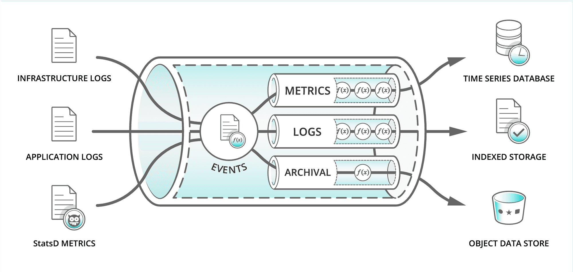
Connectivity and automation led to increased dependency on complex software systems (Sensors → Embedded IoT → Phone/App → Backend/Cloud) across industries
Software continuously updated independently of other dependent components.
Static pre-defined data schema not scalable in large software systems
A point of sale SQLite database should flexibly handle scanned data, adapting to changes in data structure without schema updates.

 Sunday
 Friday
 Monday
flowchart LR

  %% Producers
  subgraph PROD[Producers]
    PUMA[Puma SQL 🛢️]
    NIKE[Nike SQL 🛢️]
  end

  %% Backend
  subgraph BE[Backend Service]
    API[Backend API]
  end

  %% Frontend
  subgraph FE[Frontend Phone App]
    APP[Mobile App]
    LDB[Local SQL DB 🛢️]
  end

  %% Data flows
  PUMA -->|JSON feed| API
  NIKE -->|JSON feed| API

  APP <--> |JSON requests/responses| API

  APP -->|SQL queries| LDB

  API -->|Sync JSON| APP
  APP -->|Send JSON| API
{
  "product": "t-shirt",
  "brand": "Puma",
  "size": "M",
  "price": 29.99,
  "stock": 120,
  "color": "orange"   ← added today
}
INSERT INTO products
  (product, brand, size, price, stock, color)
VALUES
  ('t-shirt', 'Puma', 'M', 29.99, 120, 'orange');
⚠️ Mismatch:
JSON has "color"
Table has no "color" column

ERROR: column "color"
does not exist
flowchart TB
    SQL[SQL Queries] --> RDBMS[(Relational DB)]
    S1[awk] --> RDBMS
    S2[sed] --> RDBMS
    S3[grep] --> RDBMS
flowchart TB
  MQL[MQL MongoDB] --> DB[NoSQL Data Stores]
  GraphQL[GraphQL] --> DB
  JSIDB[JavaScript IndexedDB] --> DB
  Redis[Redis Commands] --> DB
  CQL[CQL Cassandra] --> DB
| Example | RDBMS Limitation |
|---|---|
| FB: ~4 PB/day | No horizontal scaling |
| IoT sensors: TB/hour | Storage bottlenecks |
| Example | RDBMS Limitation |
|---|---|
| NYSE: ms updates | No real-time support |
| Twitter: 6K tweets/sec | Slow insert rate |
| Example | RDBMS Limitation |
|---|---|
| Logs, images, JSON | Strict schemas only |
| Emails, videos | No native support |
| Example | RDBMS Limitation |
|---|---|
| User-entered data | Rejects nulls/invalid |
| Web scraping | Requires clean data |
| Example | RDBMS Limitation |
|---|---|
| ML pipelines | No parallel compute |
| BigQuery/Spark jobs | Slow joins & scans |
items
idby_name, by_price
{
  id: 1,
  name: "Chair",
  price: 49,
  stock: 10
}itemsCREATE TABLE items (
id INTEGER PRIMARY KEY,
name TEXT,
price REAL,
stock INTEGER
);(1, 'Chair', 49, 10)// CREATE
store.add({id: 1, name: "Chair", price: 49, stock: 10});
// READ
store.get(1);
// UPDATE
store.put({id: 1, name: "Chair", price: 59, stock: 10});
// DELETE
store.delete(1);
-- CREATE
INSERT INTO items VALUES (1, 'Chair', 49, 10);

-- READ
SELECT * FROM items WHERE id = 1;

-- UPDATE
UPDATE items SET price = 59 WHERE id = 1;

-- DELETE
DELETE FROM items WHERE id = 1;

flowchart LR
  subgraph TAB["Browser Tab (JavaScript)"]
    A["async call → Promise"]
    B["await (until resolve)"]
  end

  subgraph PROC["Browser Process"]
    IDB["IndexedDB backend"]
    STOR["Storage service"]
  end

  subgraph OS["Operating System"]
    FS["File System (disk I/O)"]
  end

  A --> IDB
  B -.-> A
  IDB --> STOR --> FS
  FS --> STOR --> IDB
  IDB -->|"completion event"| A
flowchart TB
  BPROC["Browser Process"]
  TAB1["Tab 1: Renderer
(sandboxed)"]
  TAB2["Tab 2: Renderer
(sandboxed)"]
  DB["IndexedDB Storage
(per-origin, on disk)"]

  BPROC --> TAB1
  BPROC --> TAB2

  TAB1 -->|async request| DB
  TAB2 -->|async request| DB
%%{init: {'flowchart': { 'htmlLabels': true, 'useMaxWidth': true, 'wrap': true, 'curve': 'linear', 'nodeSpacing': 40, 'rankSpacing': 60 }}}%%
flowchart TB

classDef box fill:#eef,stroke:#333,stroke-width:1px,color:#000;
classDef os  fill:#fffdcc,stroke:#333,stroke-width:1px,color:#000;

APP["Layer 7: Application
(apps: browser (IndexedDB))"]:::box
OS["Operating System
(spans multiple layers)"]:::os
US["Layers 5–6
User-space libraries & services
(session, TLS, encoding)"]:::box
KRN["Layers 2–4
Kernel networking stack
(L2/L3/L4)"]:::box
HW["Layer 1: Physical
(NIC, cable, radio)"]:::box

APP --> OS
OS --> US
OS --> KRN
US --> HW
KRN --> HW

%% Explicit widths so labels never clip
style APP width:760px
style OS  width:760px
style US  width:360px
style KRN width:360px
style HW  width:760px
// Async default: does not wait
store.put({id: 1, name: "Chair"});
let item = store.get(1);   // ❌ may run before put finishes

// Correct with await
await store.put({id: 1, name: "Chair"});
let item = await store.get(1); // ✅ read after write
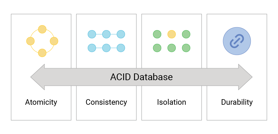
| Property | Meaning | IndexedDB |
|---|---|---|
| Atomicity | All operations in a transaction succeed or all fail. | Yes: transactions are atomic. |
| Consistency | Database moves from one valid state to another. | Yes: enforced within a transaction. |
| Isolation | Concurrent transactions do not interfere. | Partial: isolation within one tab, but multiple tabs can interfere. |
| Durability | Once committed, data persists even after crash/power loss. | Yes: backed by disk storage. |
// Open DB
const req = indexedDB.open("furnitureDB", 1);

req.onupgradeneeded = e => {
  let db = e.target.result;
  db.createObjectStore("items", { keyPath: "id", autoIncrement: true });
};

req.onsuccess = e => {
  let db = e.target.result;
  let tx = db.transaction("items", "readwrite");
  let store = tx.objectStore("items");
  store.add({ name: "Chair" });   // Insert one record each page load
};
let tx = db.transaction("items", "readwrite");
let store = tx.objectStore("items");

let req = store.get(1); // Check first

req.onsuccess = e => {
  if (e.target.result) {
    store.put({ id: 1, name: "Chair" }); // Record exists → update
  } else {
    store.add({ id: 1, name: "Chair" }); // Not found → insert
  }
};
// Create store with primary key
let store = db.createObjectStore("items", {
  keyPath: "id", autoIncrement: true
});

// Primary key "id" is automatically indexed
store.add({ name: "Chair", price: 49 });

// Fast lookup by id
store.get(1);  // uses the implicit index

const req = indexedDB.open("furnitureDB", 1);
req.onupgradeneeded = e => {
  let db = e.target.result;
  let store = db.createObjectStore("items", {
    keyPath: "id"
  });
  store.createIndex("by_name", "name", {
    unique: true
  });
};
let tx = db.transaction("items", "readonly");
let store = tx.objectStore("items");
let idx = store.index("by_name");
let req = idx.get("Chair");


erDiagram
  CUSTOMER ||--o{ ORDER : places
  PRODUCT ||--o{ ORDER : included_in

  CUSTOMER {
    int id
    string name
    string email
  }
  PRODUCT {
    int id
    string name
    float price
  }
  ORDER {
    int id
    date order_date
    int product_id
    int quantity
  }
| OrderID (PK) | Customer | Products |
|---|---|---|
| 101 | Alice | Chair, Table |
| 102 | Bob | Sofa |
In 1NF, Products column would be split so each row has a single product.
SELECT * FROM Customer;

SELECT c.name, o.order_date FROM Customer c
JOIN Order o ON c.id = o.customer_id;

SELECT p.name, SUM(o.quantity) AS total_sold FROM Order o
JOIN Product p ON o.product_id = p.id
GROUP BY p.name;
classDiagram
  class Customer {
    +int id
    +string name
    +string email
    +placeOrder(product, qty)
  }
  class Order {
    +int id
    +date orderDate
    +addItem(product, qty)
    +getTotal()
  }
  class Product {
    +int id
    +string name
    +float price
  }

  Customer "1" o-- "*" Order : places
  Order "*" *-- "*" Product : items
// ❌ Before
const order = { items: [] };
order.items.push({ name:"Chair", price:50 });
console.log(order.items[0].price);

// ✅ After
class Order {
  constructor(){ this.items=[]; }
  add(p){ this.items.push(p); }
}

const o = new Order();
o.add({ name:"Chair", price:50 });
console.log(o.items[0].price);
order.total())
class Order {
  constructor(){ this.items=[]; }
  add(p, q){ this.items.push({p,q}); }
  get total(){ return this.items
    .reduce((s,i)=>s+i.p.price*i.q,0); }
}

const o = new Order();
o.add({name:"Chair",price:50},2);
console.log(o.total); // query object

const customer = {
  id: 1,
  name: "Alice",
  orders: [
    { id: 101, product: "Chair", qty: 2 },
    { id: 102, product: "Table", qty: 1 }
  ]
};
console.log(customer.name);
// Denormalized
{
  "id": 1,
  "name": "Alice",
  "orders": [
    { "product": "Chair", "qty": 2 },
    { "product": "Table", "qty": 1 }
  ]
}

// Normalized
{
  "customers": [{ "id": 1, "name": "Alice" }],
  "orders": [
    { "id": 101, "customerId": 1, "product": "Chair", ... },
    { "id": 102, "customerId": 1, "product": "Table", ... }
  ]
}
{
  "customer": {
    "id": 1,
    "name": "Alice",
    "email": "alice@example.com",
    "orders": [
      {
        "id": 101,
        "order_date": "2025-09-01",
        "items": [
          { "product": "Chair", "price": 49.99,... },
          { "product": "Table", "price": 199.99,... }
        ]
      }
    ]
  }
}
// Query JSON directly
const data = {
  customer: { name: "Alice" },
  orders: [ { product:"Chair", qty:2 } ]
};

console.log(data.customer.name); // "Alice"
console.log(data.orders[0].product); // "Chair"
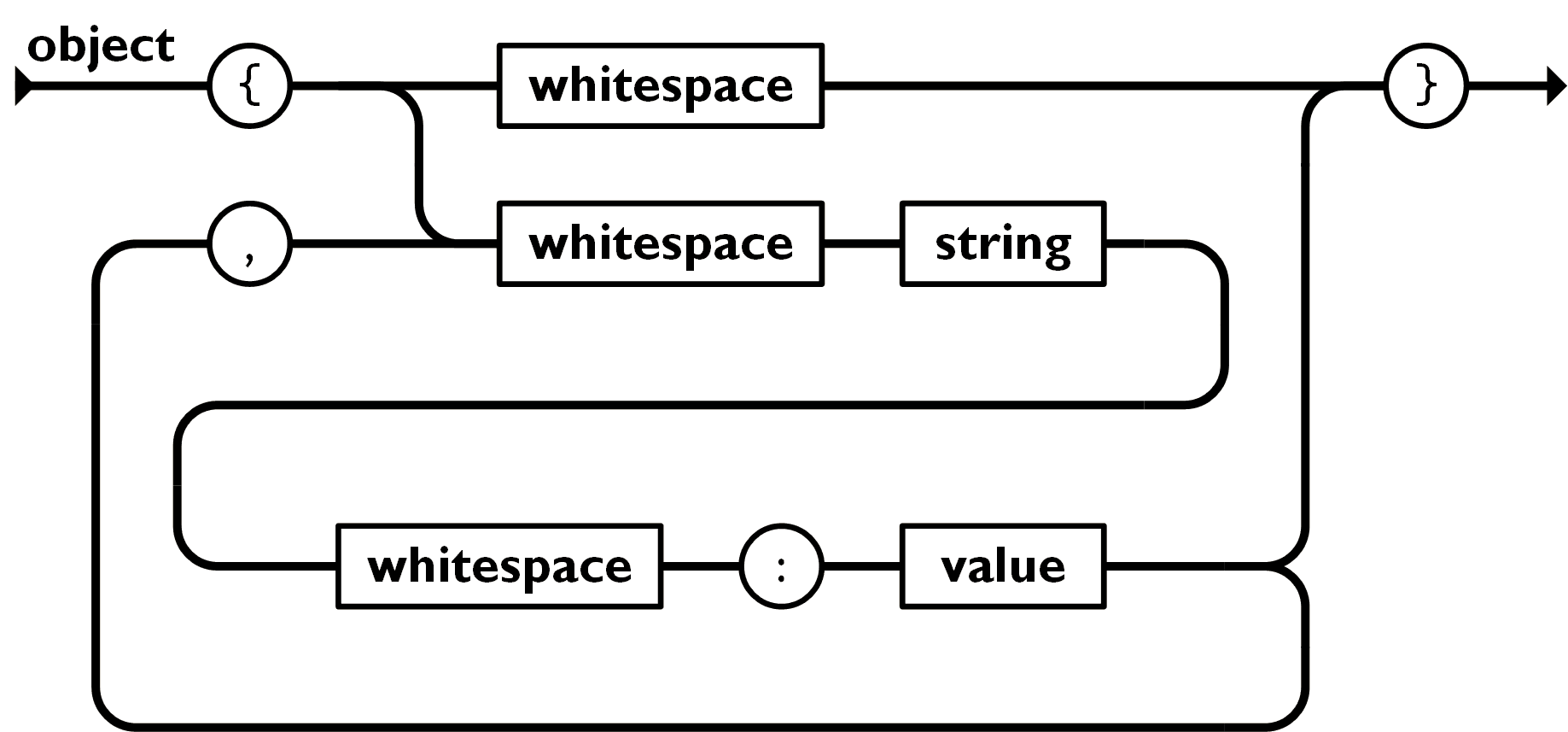
{ }
const customer = {
  id: 1,
  name: "Alice",
  email: "alice@example.com"
};
console.log(customer.name); // Alice
[ ]
const products = [
  "Chair",
  "Table",
  "Sofa"
];
console.log(products[1]); // Table
\
const message = {
  text: "Hello, World!",
  escaped: "Line1\nLine2"
};
console.log(message.text);
true / false
const order = {
  qty: 2,
  price: 49.99,
  available: true
};
console.log(order.price * order.qty); // 99.98
null
const profile = {
  name: "Alice",
  note: null
};
console.log(profile.note); // null
Is each snippet valid JSON?
1. { "name": "Alice" }
2. { name: "Alice" }
3. { "age": 25, }
4. [ "red", "green", "blue" ]
5. [ "a", "b",, "c" ]
6. { "valid": true, "value": null }
7. { "price": 19.99, "qty": 2 }
8. { "flag": True }
9. { "nested": { "x": 1, "y": 2 } }
10. "Just a string"
{
  "customer_id": 1,
  "customer_name": "Alice",
  "order_id": 101,
  "product": "Chair",
  "qty": 2
}
{
  "customer": {
    "id": 1,
    "name": "Alice"
  },
  "order": {
    "id": 101,
    "item": {
      "product": "Chair",
      "qty": 2
    }
  }
}
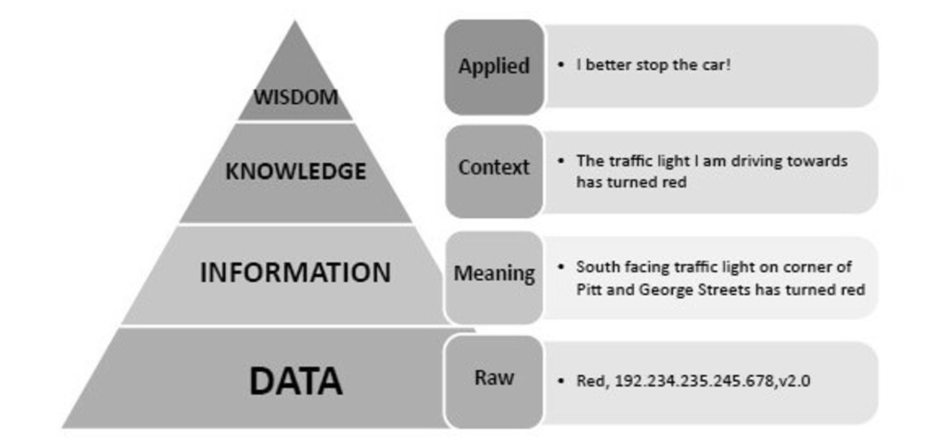
{
  "Wisdom": {
    "Knowledge": {
      "Information": {
        "Data": [
          "leaf1",
          "leaf2",
          "leaf3"
        ]
      }
    }
  }
}
Model JSON requirements:
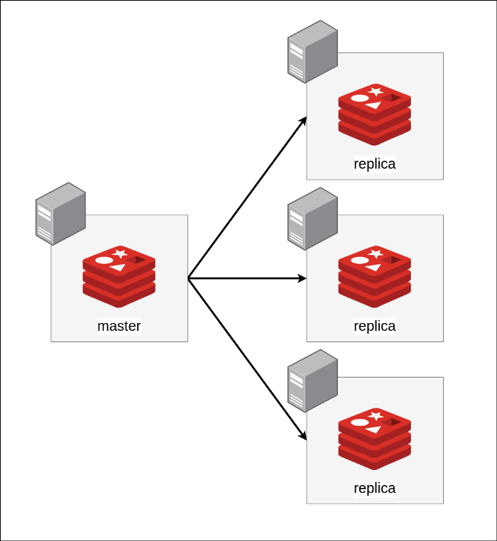
Data is stored across multiple machines for scalability, fault tolerance, and availability.
// ✅ Good ID
{ "id": "7f8c9d12", "name": "Alice" }

// ❌ Bad ID (meaning encoded)
{ "id": "2025-student-Alice", "name": "Alice" }
🔑 Every object shouldhave a unique id
This ensures:
{
  "id": "a12f-34cd-56ef",
  "name": "...",
  "type": "...",
  "createdAt": "...",
  "otherField": "..."
}
// Built-in in modern browsers
const id = crypto.randomUUID();

console.log(id);
// e.g. "3b241101-e2bb-4255-8caf-4136c566a962"
UUIDs prevent collisions across distributed systems without coordination.
  123e4567-e89b-12d3-a456-426614174000
  └───────┘ └───┘ └──┘ └──┘ └────────┘
   Time     Ver   Seq  Var   Node/Random
| Version | Basis | Notes |
|---|---|---|
| v1 | Timestamp + MAC | First defined, 1990s |
| v2 | DCE Security | Rare, site-specific |
| v3 | MD5 Hash (Name-based) | Stable for same input |
| v4 | Random | Most common today |
| v5 | SHA-1 Hash (Name-based) | More secure than v3 |
| v6, v7, v8 | Proposed (time-ordered, Unix time, custom) | 2020s improvements |
YYYY-MM-DD → hh:mm:ss → timezone
// ISO 8601 Examples

"2025-09-04"
// date only (YYYY-MM-DD)

"2025-09-04T10:15:30Z"
// UTC time (Z = Zulu)

"2025-09-04T10:15:30-07:00"
// local time with offset
✅ Always use ISO 8601 for storing & exchanging dates
// ISO 8601 with Z

"2025-09-04T10:15:30Z"
// 10:15:30 UTC

"2025-09-04T03:15:30-07:00"
// Same moment in California (UTC-7)

"2025-09-04T12:15:30+02:00"
// Same moment in Central Europe (UTC+2)
✅ Z ensures a single global reference, independent of local timezones.

// JavaScript (Browser)
const z = new Date().toISOString();
// e.g. "2025-09-04T13:22:11.123Z"
// JavaScript (Node.js)
const z = new Date().toISOString();
# Python 3
from datetime import datetime, timezone
z = datetime.now(timezone.utc).isoformat()
# e.g. "2025-09-04T13:22:11.123456+00:00"
# Ruby
require "time"
z = Time.now.utc.iso8601
// Java (java.time)
import java.time.*;
String z = Instant.now().toString();
// or:
String z2 = OffsetDateTime.now(ZoneOffset.UTC).toString();
// Go
import "time"
z := time.Now().UTC().Format(time.RFC3339)
// C#
string z = DateTime.UtcNow.ToString("o");
// ISO 8601, e.g. 2025-09-04T13:22:11.1234567Z
// PHP
$z = (new DateTime('now', new DateTimeZone('UTC')))
       ->format(DateTime::ATOM);
# Shell (Unix)
date -u +"%Y-%m-%dT%H:%M:%SZ"
Tip: Prefer ISO 8601 strings (with Z) when storing or exchanging timestamps.
Embed when:
{
  "userId": "u1",
  "name": "Alice",
  "address": {
    "city": "Stockton",
    "zip": "95211"
  }
}
Reference when:
// 1 → n (one user in multiple groups)
{ "userId": "u1", "groupIds": ["g1", "g2"] }

// n ↔ n (mutual references between users & groups)
{ "userId": "u2", "groupIds": ["g1"] }

{ "groupId": "g1", "memberIds": ["u1", "u2"] }
// Store authorName directly with posts
{
  "postId": "p1",
  "title": "JSON Best Practices",
  "authorId": "u1",
  "authorName": "Alice"
}
is,
has, or can
isActive, hasLicense, canEdit
List
userList, tags, orderIds
priceUSD, ageYears, timeoutMs
userName, email, addressLine
At
createdAt, updatedAt, expiresAt
userProfile, billingInfo, geoLocation
id suffix
userId, orderId, sessionId
{
  "userId": "u123",
  "userName": "Alice",
  "isActive": true,
  "tags": ["student", "premium"],
  "orderIds": ["o1001", "o1002"],
  "priceUSD": 199.99,
  "createdAt": "2025-09-04T10:15:00Z",
  "userProfile": {
    "ageYears": 29,
    "email": "alice@example.com"
  }
}✅ Common fields for metadata object:
{
  "metadata": {
    "createdAt": "2025-09-04T12:00:00Z",
    "updatedAt": "2025-09-04T12:30:00Z",
    "author": "u1", // source device
    "tags": ["json", "nosql", "big-data"],
    "status": "active",
    "checksum": "a1b2c3d4",
    "permissions": {
      "read": ["admin", "editor"],
      "write": ["admin"]
    }
  }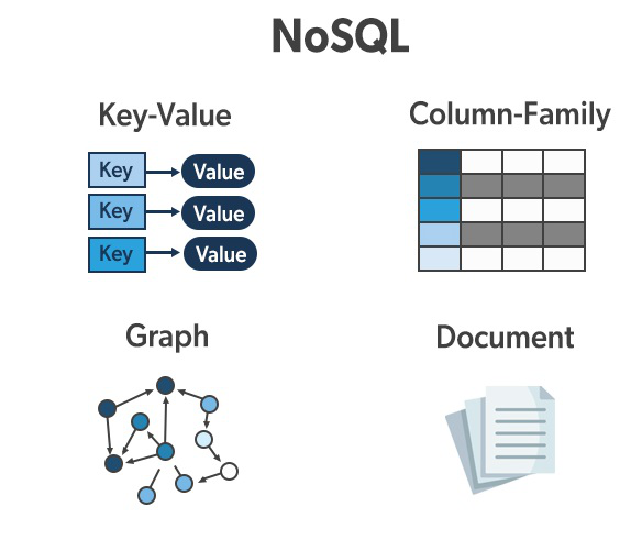
}| Database | Type | Query Language | Data Format | ACID | CAP | |||||
|---|---|---|---|---|---|---|---|---|---|---|
| A | C | I | D | C | A | P | ||||
| IndexedDB | Key-Value (browser) | JavaScript API | JSON | ✓ | ✓ | ✓ | ✓ | |||
| MongoDB | Document Store | |||||||||
| Neo4j | Graph Database | |||||||||
| Cassandra | Wide-Column Store | |||||||||
| Reddis | Key-Value (in-memory) | |||||||||
| ClickHouse | Columnar (OLAP) | |||||||||
| FAISS | Vector Index / Library | |||||||||
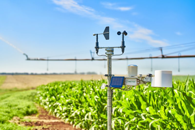
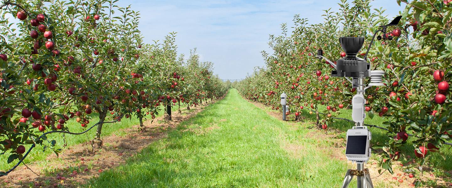
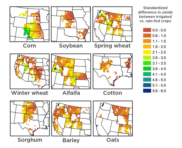
In this lab, you will develop a web application that collects and stores unstructured agricultural data using IndexedDB. You will implement functionality to handle various data types, including sensor readings, images, farmer notes, GPS coordinates, and timestamps

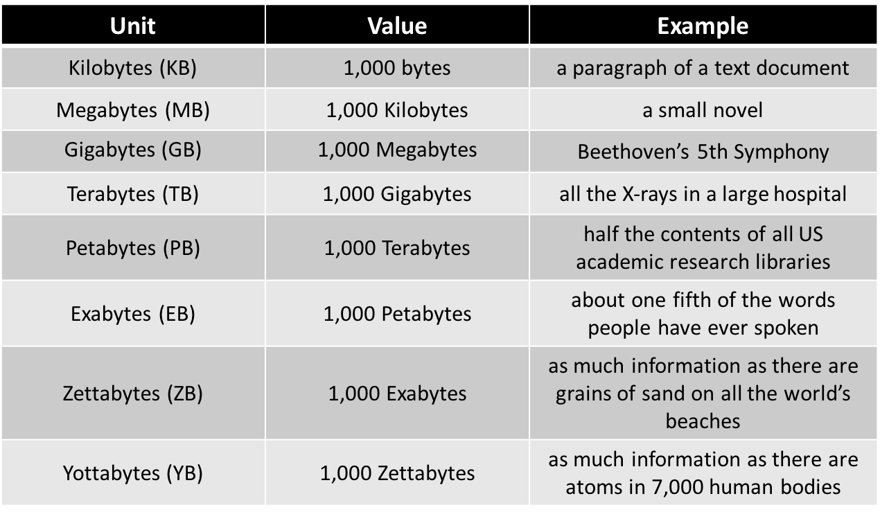
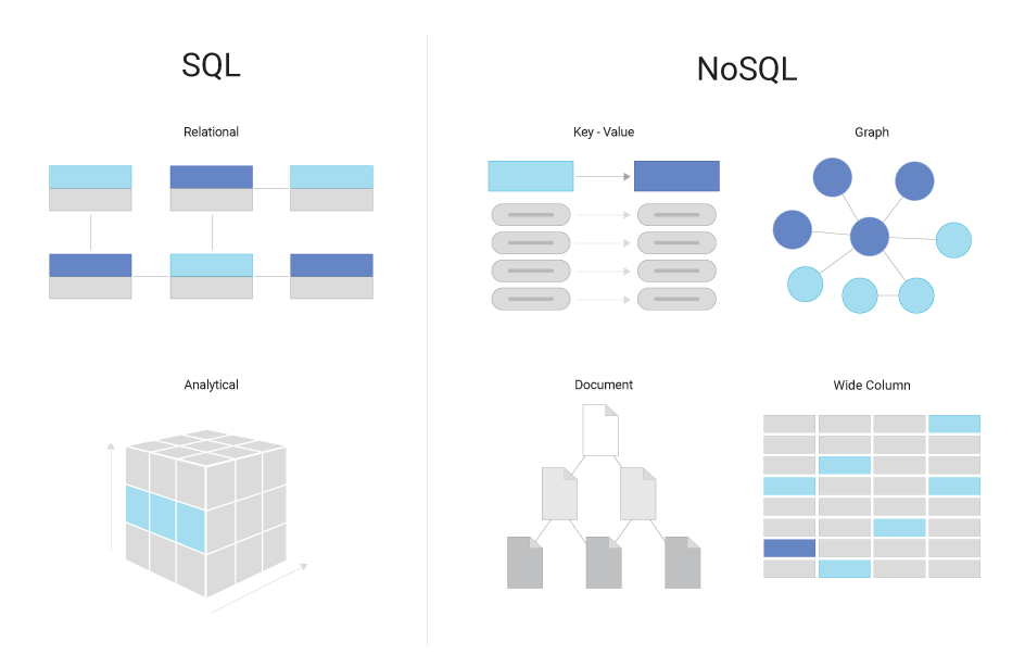
NoSQL, Key-Value Store, Document Store, Column Store, Graph Database, CAP Theorem, BASE Model, ACID Properties, Eventual Consistency, Strong Consistency, Sharding, Replication, Partitioning, Horizontal Scaling, Vertical Scaling, Consistency, Availability, Partition Tolerance, Vector Clock, Schema-less, Indexing, Secondary Index, Primary Key, Unique Index, Compound Key, MapReduce, Aggregation, Query Engine, Query Planner, Execution Plan, CRUD, Insert, Update, Delete, Read, Transaction, Object Store, Async I/O, Promise, Await, Sandbox, Same-Origin Policy, JSON, BSON, Data Lake, Data Warehouse, ETL, ELT, Streaming, Batch Processing, Lambda Architecture, Kappa Architecture, Pub/Sub, Message Queue, Idempotency, Conflict Resolution, Event Sourcing, CQRS, Distributed Cache, Sharding, Replication, In-Memory Database, Time-Series Database, Search Index, Inverted Index, Full-Text Search, 5 Vs of Big Data: Volume, Velocity, Variety, Veracity, Value.
Write a local offline database using IndexedDB to keep track of books borrowed from a library.


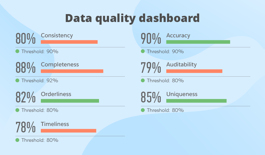
The quality of the data
determines the quality
of the software.


| Accuracy | Completeness | Consistency |
| Timeliness | Validity | Uniqueness |
| Integrity | ||
// ✅ Consistent
{ "id": 1, "unit": "kg" }
{ "id": 2, "unit": "kg" }

// ❌ Inconsistent
{ "id": 3, "unit": "kg" }
{ "id": 4, "unit": "lbs" }
// ✅ Accurate
{ "crop": "Wheat", "yieldKg": 7200 }

// ❌ Inaccurate (too high to be realistic)
{ "crop": "Wheat", "yieldKg": 7200000 }
// ✅ Complete
{ "id": 1, "crop": "Maize", "soil": "Loam" }

// ❌ Incomplete (missing soil)
{ "id": 2, "crop": "Maize" }
// ✅ Timely
{ "crop": "Rice", "updatedAt": "2025-09-08T09:00Z" }

// ❌ Outdated
{ "crop": "Rice", "updatedAt": "2020-05-01T10:00Z" }
// ✅ Unique IDs
{ "id": 1, "crop": "Barley" }
{ "id": 2, "crop": "Millet" }

// ❌ Duplicate IDs
{ "id": 3, "crop": "Wheat" }
{ "id": 3, "crop": "Wheat" }
// ✅ Valid
{ "id": 10, "organic": true, "harvestDate": "2025-09-01" }

// ❌ Invalid (wrong type + bad date)
{ "id": "ten", "organic": "yes", "harvestDate": "jan-2025" }
// ✅ With integrity
{ "farmId": 1, "cropId": 101, "crop": "Maize" }
{ "cropId": 101, "name": "Maize" }

// ❌ Broken reference (farm points to missing crop)
{ "farmId": 2, "cropId": 999, "crop": "Unknown" }
How to validate data quality?

How to validate data quality?

// MongoDB
db.farm.find({ yieldKg: { $lt: 0 } })

// SQL
SELECT * FROM farm
WHERE yield_kg < 0;
Type: SHA-256
# Python
import hashlib

with open('data.txt', 'rb') as f:
    bytes = f.read()
    hash = hashlib.sha256(bytes).hexdigest()
    # Example output: 3a7bd3e2360a...
    print(hash)
Type: SHA-256
// JavaScript (Node.js)
const crypto = require('crypto');
const fs = require('fs');

const fileBuffer = fs.readFileSync('data.txt');
const hash = crypto.createHash('sha256')
                   .update(fileBuffer)
                   .digest('hex');
// Example output: 3a7bd3e2360a...
console.log(hash);
{
  "meta": {
    "checksum": "3a7bd3e2360a9e3f2a1c4b..."
  },
  "data": {
    "sensorId": "S1001",
    "temperature": 22.5,
    "humidity": 45,
    "timestamp": "2025-09-08T15:00:00Z"
  }
}

// MongoDB
db.farm.find({
  season:{ $nin:["Spring","Fall"] }
})

// SQL
SELECT * FROM farm
WHERE season NOT IN
 ('Spring','Fall');
{
  "id": 1,
  "crop": "Wheat",
  "yieldKg": 7500,
  "harvestDate": "32-13-2025",
  "price": 250,
  "irrigation": "Drip",
  "stock": 120,
  "locaton": "Field A",
  "owner": 12345,
  "organic": "maybe"
}
// MongoDB: find docs where 'organic' is not boolean
db.farm.find({
  $expr: { $ne: [ { $type: "$organic" }, "bool" ] }
})
Consistency • Accuracy • Completeness • Timeliness • Uniqueness
➡️ Thursday
{
  "id": 42,
  "crop": "Wheat",
  "yieldKg": 7200,
  "unit": "lbs",
  "owner": "Alice",
  "harvestDate": "13/31/2025",
  "updatedAt": "2022-01-10T10:00:00Z"
}
❌ Metrics not met:
- Consistency
- Validity
- Timeliness
Note: The name MongoDB comes from "humongous" (meaning huge).


{
  "_id": ObjectId("64f9c1a2b1234c5678d90ef1"),
  "crop": "Wheat",
  "yieldKg": 7500,
  "irrigation": "Drip",
  "location": { // No joins needed
    "field": "North",
    "soil": "Loam"
  },
  "farmerName": "John Doe",
  "farmerPhone": "555-1234",
  "equipmentUsed": "Tractor-101",
  "marketPriceUSD": 250
}SQL (Normalized):
-- Crops table
Crops(id, crop, yieldKg, irrigation, locationId)

-- Location table
Locations(id, field, soil)

-- Farmers table
Farmers(id, name, phone)

-- Equipment table
Equipment(id, name)
✅ Avoids duplication, but needs joins to query.
MongoDB (Denormalized):
{
  "_id": ObjectId("64f9c1a2b1234c5678d90ef1"),
  "crop": "Wheat",
  "yieldKg": 7500,
  "irrigation": "Drip",
  "location": { "field": "North", "soil": "Loam" },
  "farmer": { "name": "John Doe", "phone": "555-1234" },
  "equipmentUsed": ["Tractor-101", "Seeder-202"]
}
⚡ All info in one document → fast reads, but duplicates farmer/equipment across docs.
// Document
{ crop:"Wheat",yieldKg:3000,
  soil:"Loam" }
{
  "farm": "GreenField",
  "crop": "Wheat",
  "year": 2024,
  "yield_tons": 120,
  "location": "California"
}
// Find farms growing Wheat
db.crops.find({
    crop: "Wheat"
});
// Principles of MQL
- JSON-like syntax
- Expressive operators ($gt, $set, etc.)
- CRUD: Create, Read, Update, Delete
- Works locally or in Atlas
// Find all wheat crops
db.crops.find(
  { crop: "Wheat" },          // filter
  { crop: 1, yieldKg: 1 }     // projection
)
// Find with range filter
db.crops.find(
  { yieldKg: { $gt: 5000 } }, // filter
  { crop: 1, irrigation: 1 }  // projection
)
Reference: MongoDB Query Language (MQL) Documentation
// Example: Find crops with yield > 5000
db.crops.find(
  { yieldKg: { $gt: 5000 } },   // filter
  { crop: 1, yieldKg: 1 }       // projection
)
{
  "_id": ObjectId("650f5a2e1c4d3a6b7f9d1234"),
  "name": "Rose",
  "color": "Red",
  "weightInKg": 0.5,
  "timestamp": ISODate("2025-09-08T15:00:00Z")
}
// Insert query
const insertResult = db.flowers.insertOne({
  name: "Tulip",
  color: "Yellow"
});

// Output:
// {
//   acknowledged: true,
//   insertedId: ObjectId("f9d5678...")
// }
// SQL
CREATE TABLE farm (
    id INT PRIMARY KEY AUTO_INCREMENT,
    crop VARCHAR(50)
);

INSERT INTO farm(crop)
VALUES ('Rice');
// MongoDB
use farmDB
db.createCollection("farm")
db.farm.insertOne({ crop:"Rice" })
// SQL
SELECT *
FROM farm
WHERE crop = 'Rice';
// MongoDB
db.farm.find({ crop: "Rice" })
// SQL
UPDATE farm
SET yield_kg = 4000
WHERE crop = 'Rice';
// MongoDB
db.farm.updateOne(
    { crop: "Rice" },
    { $set: { yieldKg: 4000 } }
)
// SQL
DELETE FROM farm
WHERE crop = 'Rice';
// MongoDB
db.farm.deleteOne({ crop: "Rice" })
// MongoDB
db.farm.find({yieldKg:{$gt:3000}})

// SQL
SELECT * FROM farm
WHERE yield_kg>3000;
// MongoDB
db.farm.find({$and:[
 {crop:"Wheat"},{yieldKg:{$gt:2000}}]})

// SQL
SELECT * FROM farm
WHERE crop='Wheat' AND yield_kg>2000;
// MongoDB
db.farm.find({crop:/^W/})

// SQL
SELECT * FROM farm
WHERE crop LIKE 'W%';
// SQL
SELECT * FROM farm
WHERE yield_kg > 6000;
// MongoDB
db.farm.find({ yieldKg: { $gt: 6000 } })
// SQL
SELECT * FROM farm
WHERE irrigation IS NULL;
// MongoDB
db.farm.find({ irrigation: null })
// SQL
SELECT *
FROM farm
ORDER BY price ASC
LIMIT 1;
// MongoDB
db.farm.find().sort({ price: 1 }).limit(1)
// SQL
UPDATE farm
SET stock = stock + 20
WHERE crop = 'Maize';
// MongoDB
db.farm.updateOne(
    { crop: "Maize" },
    { $inc: { stock: 20 } }
)
// SQL
DELETE FROM farm
WHERE yield_kg < 1000;
// MongoDB
db.farm.deleteMany(
    { yieldKg: { $lt: 1000 } }
)
How to validate data quality?
| Accuracy | Completeness | Consistency |
| Timeliness | Validity | Uniqueness |
| Integrity | ||
// Validity
// Enforce required fields
db.createCollection("readings", {
  validator: {
    $jsonSchema: {
      // Completeness
      required: ["deviceId", "ts"]
    }
  }
})
// Validity, Accuracy
properties: {
  deviceId: { bsonType: "string" },
  ts: { bsonType: "date" },
  moisture: { minimum: 0, maximum: 100 },
  unit: { enum: ["percent"] }
}
// Validity
properties: {
  deviceId: { bsonType: "string" },
  ts: { bsonType: "date" },
  moisture: { bsonType: "double" }
}
// Consistency
properties: {
  battery: { bsonType: "int" },
  healthy: { bsonType: "bool" },
  tags: { bsonType: "array" },
  meta: { bsonType: "object" }
}
// Normalize on write
db.readings.updateOne(
  { deviceId: "plant-007", ts: ts },
  {
    $set: {
      unit: "percent",
      moisture: { $toDecimal: "$moisture" }
    }
  },
  { upsert: true }
)
db.readings.updateOne(
  { deviceId: "plant-007", ts: ts },
  {
    $set: {
      battery: { $ifNull: ["$battery", 100] }
    }
  },
  { upsert: true }
)
db.readings.updateMany(
  {},
  [{ $set: {
    deviceId: { $toString: "$deviceId" },
    ts: { $toDate: "$ts" },
    moisture: { $toDecimal: "$moisture" },
    battery: { $ifNull: ["$battery", 100] }
  }}]
)
db.readings.updateMany(
  {},
  [{ $set: {
    unit: "percent",
    healthy: { $toBool: "$healthy" },
    count: { $toInt: "$count" },
    tags: { $ifNull: ["$tags", []] },
    meta: { $ifNull: ["$meta", {}] }
  }}]
)
{
  deviceId: 12345,
  ts: "2025-09-11",
  moisture: "42",
  battery: null,
  healthy: "true"
}
{
  deviceId: "12345",
  ts: ISODate("2025-09-11T00:00:00Z"),
  moisture: NumberDecimal("42"),
  battery: 100,
  healthy: true,
  tags: [],
  meta: {}
}
// Uniqueness
db.readings.createIndex(
  { deviceId: 1, ts: 1 },
  { unique: true }
)
// Accuracy, Validity
db.readings.find({
  $or: [
    { moisture: { $lt: 0 } },   // Accuracy
    { moisture: { $gt: 100 } }  // Validity
  ]
})
// Validity, Uniqueness
db.readings.createIndex(
  { deviceId: 1, ts: 1 },
  {
    unique: true,
    partialFilterExpression: {
      deviceId: { $exists: true },
      ts: { $type: "date" }
    }
  }
)
// Integrity, Accuracy
const r = db.readings.findOne(
  { deviceId: "plant-007" },
  { sort: { ts: -1 } }
)

if (!r || r.moisture < 0 || r.moisture > 100) {
  throw "Invalid input"
}
// Accuracy, Completeness
db.readings.aggregate([
  { $match: { unit: "percent" } },
  { $group: {
      _id: "$deviceId",
      avgMoisture: { $avg: "$moisture" },
      minMoisture: { $min: "$moisture" },
      maxMoisture: { $max: "$moisture" },
      totalReadings: { $sum: 1 },
      count: { $count: {} }
])
// Accuracy, Completeness
db.readings.aggregate([
  { $group: {
      _id: null,
      nullMoisture: { $sum: {
        $cond: [{$eq:["$moisture",null]},1,0] }},
      outOfRange:   { $sum: {
        $cond: [
            {
                $or:[{$lt:["$moisture",0]},
                {$gt:["$moisture",100]}]},1,0
        ]}}
  }}
])
// Integrity
db.audit.insertOne({
  action: "UPDATE",
  target: "readings",
  ts: new Date(),
  user: "system",
  changes: { field: "moisture", old: "42", new: "42.0" }
})
Eventually Consistent
| Accuracy ✓ | Completeness ✓ | Consistency ✓ |
| Timeliness | Validity ✓ | Uniqueness ✓ |
| Integrity ✓ | ||
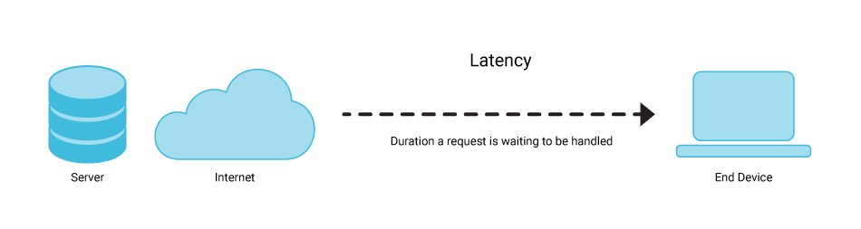
Big Data Transport Latency (100 MB)
-----------------------------------
1 Gbps : ~0.8 s one-way
100 Mbps : ~8 s one-way
10 Mbps : ~80 s one-way


Round-trip ≈ 2x + small ACK delay
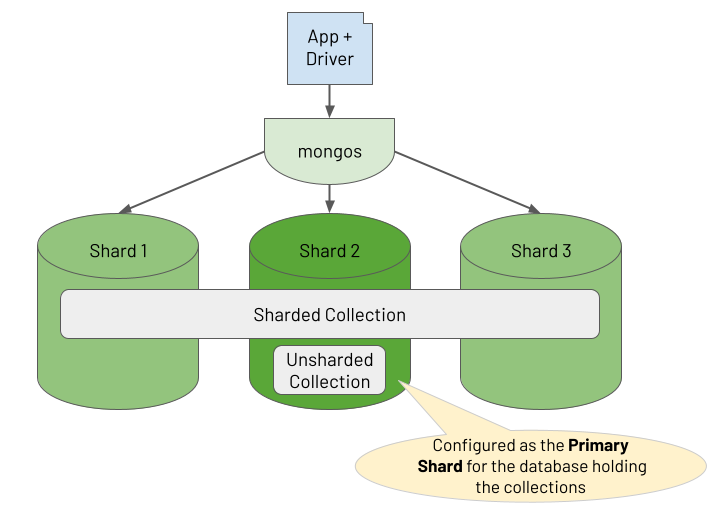
// Timeliness
// Shard readings by deviceId
db.adminCommand({
  shardCollection: "iot.readings",
  key: { deviceId: 1 }
})
// Check balancer status
db.adminCommand({ balancerStatus: 1 })

// Move chunk manually if needed
db.adminCommand({
  moveChunk: "iot.readings",
  find: { deviceId: "plant-007" },
  to: "shard0001"
})
// Example query routed by key
db.readings.find({ deviceId: "plant-007" })

// Query router (mongos)
// ensures minimal latency
// Timeliness
db.staging.createIndex(
  { expiresAt: 1 },
  { expireAfterSeconds: 0 }
)
// Timeliness
// Auto-delete 24h after ts
db.staging.createIndex(
  { ts: 1 },
  { expireAfterSeconds: 86400 }
)
// Timeliness
// Auto-delete at expiresAt
db.logs.createIndex(
  { expiresAt: 1 },
  { expireAfterSeconds: 0 }
)

db.logs.insertOne({
  msg: "debug",
  expiresAt: ISODate("2025-09-12T00:00:00Z")
})
| Accuracy ✓ | Completeness ✓ | Consistency ✓ |
| Timeliness ✓ | Validity ✓ | Uniqueness ✓ |
| Integrity ✓ | ||
In a farm databases, which data quality metricis the hardest to guarantee?

-- Filter high-yield crops
SELECT *
FROM crops
WHERE yield_per_hectare > 5000;

-- Sum total production
SELECT SUM(production_tonnes) AS total
FROM crops;

-- Update harvest_date to DATE format
UPDATE crops
SET harvest_date = DATE('2025-09-14')
WHERE id = 1;
#include <stdio.h>

int main() {
    int yields[5] = {4000, 5200, 3100};
    int total = 0;

    for (int i = 0; i < 5; i++) { // Iteration
        if (yields[i] > 5000) {   // Selection
            total += yields[i];    // Sequence
        }
    }
    printf("Total high yield = %d\n", total);
    return 0;
}

// Example: transform yields with C
#include <stdio.h>

int main() {
    int yields[5] = {4000, 5200, 3100};
    for (int i = 0; i < 5; i++) {
        if (yields[i] > 5000) {
          printf("High yield: %d\n", yields[i]);
        }
    }
    return 0;
}
-- Simple SQL query
SELECT name, price
FROM Flowers
WHERE price > 10;
-- Loop + if-then-else
FOR each flower IN Flowers:
    IF flower.price > 10 THEN
        PRINT "Expensive"
    ELSE
        PRINT "Affordable"
    END IF
END FOR

#include <stdio.h>

int main() {
    int yields[5] = {4000, 5200, 3100};
    int total = 0;

    for (int i = 0; i < 5; i++) { // Iteration
        if (yields[i] > 5000) {   // Selection
            total += yields[i];    // Sequence
        }
    }
    printf("Total high yield = %d\n", total);
    return 0;
}
Contrast: Non-declarative requires specifying both what + how (loops, indices, control flow).
const numbers = [1, 2, 3, 4];

const doubled = numbers.map(x => x * 2);
// Result: [2, 4, 6, 8]

const objects = [{id:1}, {id:2}];
const transformed = objects.map(obj => ({
    ...obj,
    value: obj.id * 10
}));
// Result: [{id:1, value:10}, {id:2, value:20}]
//Before:
[
  { "crop": "Wheat", "yield": "5000" },
  { "crop": "Corn", "yield": "4000" }
]

//After:
[
  { "crop": "Wheat", "yield": 5000 },
  { "crop": "Corn", "yield": 4000 }
]
| Map | Filter | Reduce | |
|---|---|---|---|
| IndexedDB (JS) | |||
| MongoDB (MQL) |
// Translation: English to Spanish
["Wheat","Corn"].map(c=>c==="Wheat"?"Trigo":"Maíz");

// Data Format: Local to UTC
["01/12/25"].map(d => new Date(d).toISOString());

// Type Conversion: String to Int
["5000","4000"].map(y => parseInt(y));

// Default Value: Region
[{r:null}].map(x=>({r:x.r||"Unknown"}))
Before:
[
  { "crop": "Wheat", "yield": "5000" },
  { "crop": "Corn" }
]

After Map:
[
  { "crop": "Wheat", "yield": 5000 },
  { "crop": "Corn", "yield": "missing" }
]
const data = [
  { crop: "Wheat", yield: "5000" },
  { crop: "Corn" }
];

const mapped = data.map(d => ({
  crop: d.crop,
  yield: d.yield ? parseInt(d.yield) : "missing"
}));
const data = [
  { crop: "Wheat", yield: "5000" },
  { crop: "Corn" }
];

const transformed = [];
for (let i = 0; i < data.length; i++) {
  const d = data[i];
  let yieldVal;
  if (d.yield) {
    yieldVal = parseInt(d.yield);
  } else {
    yieldVal = "missing";
  }
  transformed.push({crop:d.crop,yield:yieldVal});
}
// Before:
const data = [{ "crop": "Wheat" }];

// After:
[
  {
    "crop": "Wheat",
    "tsLastUpdate": "2025-09-15T15:00:00Z",
    "uuid": "a1b2c3-"
  }
]
const data = [
  { crop: "Wheat" },
  { crop: "Corn" }
];

const mapped = data.map(d => ({
  ...d,
  meta: {
    tsLastUpdate: new Date(),
    uuid: crypto.randomUUID()
  }
}));
const data = [
  { crop: "Wheat" },
  { crop: "Corn" }
];

const transformed = [];
for (let i = 0; i < data.length; i++) {
  const d = data[i];
  transformed.push({
    ...d,
    meta: {
      tsLastUpdate: new Date(),
      uuid: crypto.randomUUID()
    }
  });
}
| Map | Filter | Reduce | |
|---|---|---|---|
| IndexedDB (JS) | ✓ | ||
| MongoDB (MQL) |
{
  $map: {
    input: [/* array */],
    as: "element",
    in: { /* transformation */ }
  }
}
// Create a temporary collection
db.tempNumbers.insertMany([ {
     _id: 1,
     numbers: [1,2,3,4]
    }
]);

db.tempNumbers.aggregate([
  {
    $project: {
      doubled: {
        $map: {
          input: "$numbers",
          as: "n",
          in: { $multiply: ["$$n", 2] }
        }
      }
    }
  }
]);
// Result: [{_id:1, doubled: [2,4,6,8]}]
db.tempObjects.insertOne({
    _id: 1,
    objects: [{id:1},{id:2}]
});

db.tempObjects.aggregate([
  {
    $project: {
      transformed: {
        $map: {
          input: "$objects",
          as: "obj",
          in: {
            id: "$$obj.id",
            value: { $multiply: ["$$obj.id", 10] }
          }
        }
      }
    }
  }
]);
| Map | Filter | Reduce | |
|---|---|---|---|
| IndexedDB (JS) | ✓ | ||
| MongoDB (MQL) | ✓ |


array.filter(element => condition === true)// Coffee menu as objects
const drinks = [
{ name: "Espresso", price: 3 },
{ name: "Latte", price: 4 },
{ name: "Cappuccino", price: 5 }
];
// Filter: keep only Latte
const lattes = drinks.filter(drink => drink.name === "Latte");
console.log(lattes);
// [ { name: "Latte", price: 4 } ]
// Data set
const drinks = [
  { name: "Espresso", price: "3" },
  { name: "Latte", price: "4" },
  { name: "Cappuccino", price: "5" }
];

// Req 1: Filter only Cappuccino
// Data set
const drinks = [
  { name: "Espresso", price: "3" },
  { name: "Latte", price: "4" },
  { name: "Cappuccino", price: "5" }
];

// Req 2a: Map price to number
// Req 2b: Filter drinks under $5
// Data set
const drinks = [
  { name: "Espresso", price: "3" },
  { name: "Latte", price: "4" },
  { name: "Cappuccino", price: "5" }
];
const cappuccinos = drinks.filter(d => d.name === "Cappuccino");
const cheapNames = drinks
  .map(d => ({ drink: d.name, price: Number(d.price) }))
  .filter(d => d.price < 5);
// Data set
const drinks = [
  { name: "Espresso", price: "3" },
  { name: "Latte", price: "4" },
  { name: "Cappuccino", price: "5" }
];
const cappuccinos = [];
const cheapNames = [];
for (let i = 0; i < drinks.length; i++) {
  const d = drinks[i];
    if (d.name === "Cappuccino") {
    cappuccinos.push(d);
  }
  const price = Number(d.price);
  if (price < 5) {
    cheapNames.push({ drink: d.name, price: price });
  }
}
| Map | Filter | Reduce | |
|---|---|---|---|
| IndexedDB (JS) | ✓ | ✓ | |
| MongoDB (MQL) | ✓ |
// Collection: drinks
// Documents
[
  { name: "Espresso", price: "3" },
  { name: "Latte", price: "4" },
  { name: "Cappuccino", price: "5" }
]

// Req 1: Filter only Cappuccino
// Collection: drinks
// Documents
[
  { name: "Espresso", price: "3" },
  { name: "Latte", price: "4" },
  { name: "Cappuccino", price: "5" }
]

// Req 2a: Convert price to number
// Req 2b: Filter Cappuccinos under $5
// Insert sample data
db.drinks.insertMany([
  { name: "Espresso", price: "3" },
  { name: "Latte", price: "4" },
  { name: "Cappuccino", price: "5" }
])

// Req 1: Filter only Cappuccino
db.drinks.find({ name: "Cappuccino" })

// Result:
[ { name: "Cappuccino", price: "5" } ]
// Insert sample data
db.drinks.insertMany([
  { name: "Espresso", price: "3" },
  { name: "Latte", price: "4" },
  { name: "Cappuccino", price: "5" }
])

// Req 2a: Convert price to number
// Req 2b: Filter Cappuccinos under $5
db.drinks.aggregate([
  { $match: { name: "Cappuccino" } },
  { $addFields: { price: { $toInt: "$price" } } },
  { $match: { price: { $lt: 5 } } }
])

// Result:
[ { name: "Cappuccino", price: 5 } ]
| Map | Filter | Reduce | |
|---|---|---|---|
| IndexedDB (JS) | ✓ | ✓ | |
| MongoDB (MQL) | ✓ | ✓ |

array.reduce((acc, element) =>..., initValue)// Example: sum numbers
const numbers = [1, 2, 3];
const total = numbers.reduce(
(acc, n) => acc + n, 0
);
console.log(total);
// 6
// Data set
const drinks = [
  { name: "Espresso", price: 3 },
  { name: "Latte", price: 4 },
  { name: "Cappuccino", price: 5 }
];

// Total price of all drinks
const total = drinks.reduce(
  (sum, d) => sum + d.price, 0
);

console.log(total);
// 12
// Same with loop
const drinks = [
  { name: "Espresso", price: 3 },
  { name: "Latte", price: 4 },
  { name: "Cappuccino", price: 5 }
];

let total = 0;
for (let i = 0; i < drinks.length; i++) {
  total += drinks[i].price;
}

console.log(total);
// 12
// Insert data
db.drinks.insertMany([
  { name: "Espresso", price: 3 },
  { name: "Latte", price: 4 },
  { name: "Cappuccino", price: 5 }
])

// Total price of all drinks
db.drinks.aggregate([
  { $group: { total: { $sum: "$price" } } }
])

// Result:
[ { total: 12 } ]
// Total price of Cappuccino only
db.drinks.aggregate([
  { $match: { name: "Cappuccino" } },
  { $group: { _id: "$name", total: { $sum: "$price" } } }
])

// Result:
[ { _id: "Cappuccino", total: 5 } ]
| Map | Filter | Reduce | |
|---|---|---|---|
| IndexedDB (JS) | ✓ | ✓ | ✓ |
| MongoDB (MQL) | ✓ | ✓ | ✓ |


# extract.py - Example of extracting data from an API
import requests
import json

url = "https://api.weather.com/data"
response = requests.get(url)

if response.status_code == 200:
    data = response.json()
    print("Data extracted:", data)
else:
    print("Failed:", response.status_code)

# Example structure of a data lake
lake = {
    // READ ONLY
    "uuid": "123e4567-e89b-12d3-a456-426614174000",
    "item": {
        "raw_data": {
            "sensor_readings": [...],
            "logs": [...],
            "api_data": [...]
        },
        // READ AND WRITE
        "meta_data": {
            "source": "IoT sensors",
            "timestamp": "2025-09-23T08:00:00Z",
            "tags": ["temperature", "humidity"]
        }
    }
}
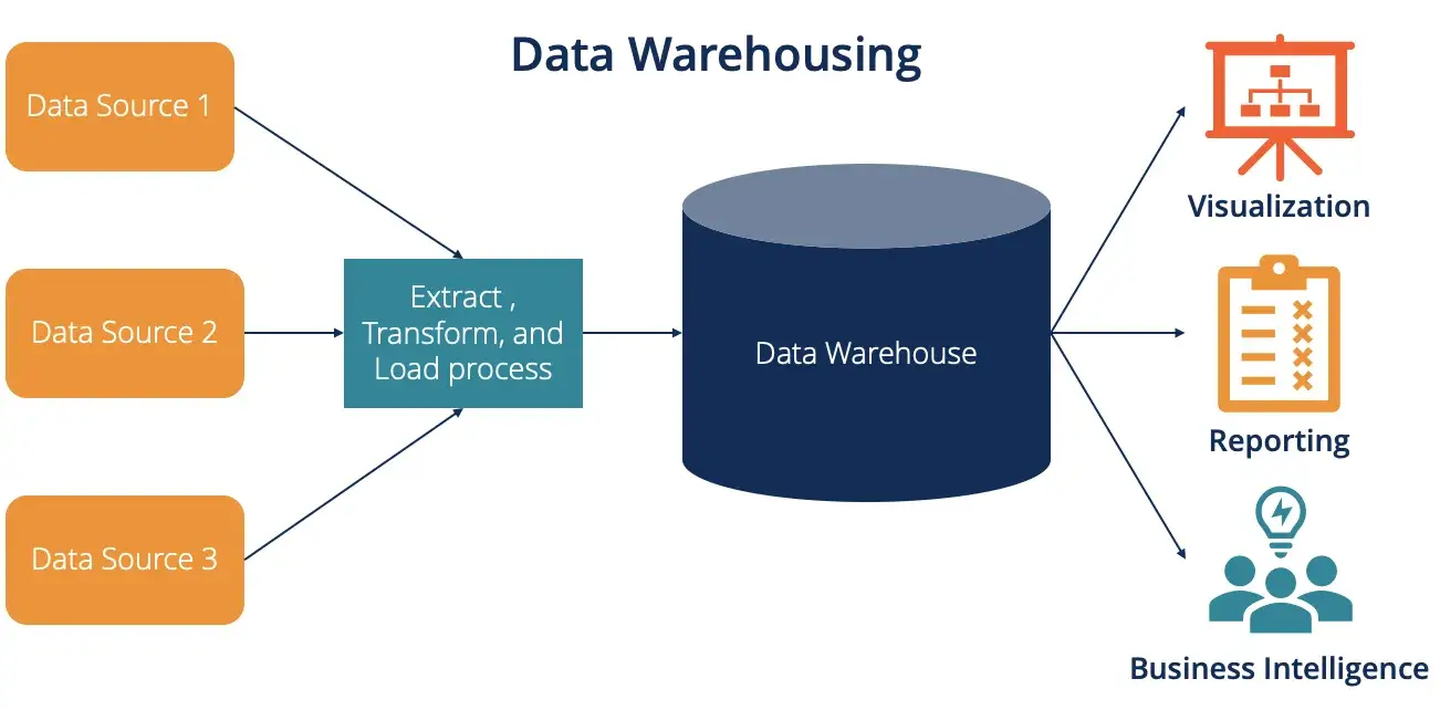
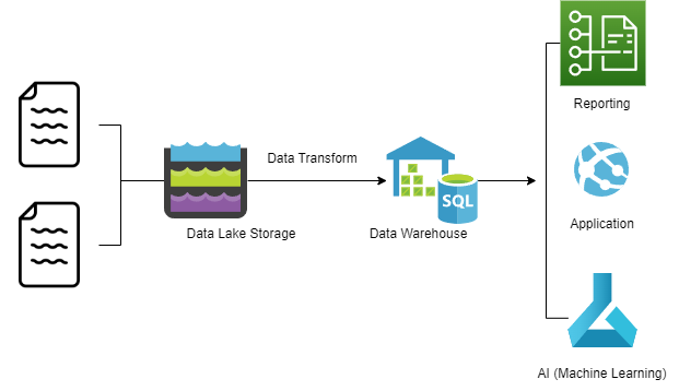
In many data pipeline architectures, the data lake is often the first and central component.
It is highly recommended to start with a data lake to ensure flexibility and scalability.

1. What is the main purpose of the Extract step in ETL?
2. Which of the following is a key characteristic of a Data Lake?
3. In ETL processes, what does the Transform step usually involve?
4. When would you recommend using ETL over ELT?


| Interval | Use Case |
|---|---|
| Real-time | IoT, fraud detection |
| Hourly | ETL jobs, logs |
| Daily | Reporting dashboards |
# etl.py - all-in-one ETL script
def etl():
    extract()
    transform()
    load()

# Separate modular files
# extract.py
def extract():
    print("Extracting data from source...")

# transform.py
def transform():
    print("Transforming and enriching data...")

# load.py
def load():
    print("Loading data into target system...")
| Type | Pros | Cons |
|---|---|---|
| Partial | Faster, less storage | Risk missing updates |
| Full | Consistent snapshot | High cost & latency |
db = MongoClient().Agriculture # connect to MongoDB
print(db.flowers.count_documents({
    "color":
        {"$exists": True}
    }))  # verify data
# Retention strategies for raw data
def retention_policy(item):
    # 1. Auto delete
    if item.age_days > 30:
        del item

    # 2. Deletion flag
    elif item.flag_for_deletion:
        item.deleted = True

    # 3. Do not delete
    else:
        pass  # keep indefinitely
# Verify checksum of metadata
doc = db.Farm.find_one({"uuid": "123e4567-e89b-..."})
meta_json = json.dumps(doc['meta_data'])
checksum = hashlib.md5(meta_json).hexdigest()

print("Stored checksum:", doc.get("checksum"))
print("Calculated checksum:", checksum)
print("Valid:", doc.get("checksum") == checksum)

1. What is a key design-time consideration when choosing ETL vs ELT?
2. Which design-time aspect involves defining cleaning, validation, and metadata?
3. Which design-time aspect determines how long raw data is kept in the pipeline?
4. When planning design-time aspects, what should you consider about data sources?
To Query Relationships
Query connections, paths, and patterns between entities.


// Create a Person node
CREATE (p:Person {name: "Alice", age: 30})
RETURN p;
// Create FRIEND relationship
MATCH (a:Person {name:"Alice"}),(b:Person {name:"Bob"})
CREATE (a)-[:FRIEND]->(b)
RETURN a, b;
// Find all Person nodes
MATCH (p:Person)
RETURN p;

// Sample return object
{
  "p": {
    "name": "Alice",
    "age": 30,
    "email": "alice@example.com"
  }
}
// Filter by age
MATCH (p:Person)
WHERE p.age > 25
RETURN p;

// Sample return objects
[
  {"name": "Alice", "age": 30},
  {"name": "Charlie", "age": 28}
]
// Update age
MATCH (p:Person {name: "Alice"})
SET p.age = 31
RETURN p;

// Sample return object
{"name": "Alice", "age": 31}
// Delete node
MATCH (p:Person {name: "Bob"})
DETACH DELETE p;

// No return object; node is deleted
// Count nodes
MATCH (p:Person)
RETURN count(p) AS totalPersons;

// Sample return object
{"totalPersons": 3}
// Find all FRIEND relationships
MATCH (a)-[r:FRIEND]->(b)
RETURN a.name, b.name;

// Sample return objects
[
  {"a.name": "Alice", "b.name": "Bob"},
  {"a.name": "Charlie", "b.name": "Alice"}
]
// Average age
MATCH (p:Person)
RETURN avg(p.age) AS averageAge;

// Sample return object
{"averageAge": 29.7}
// Optional FRIEND match
MATCH (p:Person)
OPTIONAL MATCH (p)-[:FRIEND]->(f)
RETURN p.name, collect(f.name) AS friends;

// Sample return objects
[
  {"p.name": "Alice", "friends": ["Bob", "Charlie"]},
  {"p.name": "Charlie", "friends": []}
]
// SQL query
SELECT f.name
FROM Person p
JOIN FRIENDS fr ON p.id = fr.person_id
JOIN Person f ON fr.friend_id = f.id
WHERE p.name = 'Alice';

// Cypher query
MATCH (a:Person {name: "Alice"})-[:FRIEND]->(f)
RETURN f.name;
| Database | Atomicity | Consistency | Isolation | Durability |
|---|---|---|---|---|
| IndexedDB | Yes | Yes | Yes (per transaction) | Yes |
| MongoDB | Yes (single document) | Yes (single document) | Limited | Yes (with journaling) |
| Neo4j | Yes | Yes | Yes | Yes |
| SQL (e.g., MySQL, PostgreSQL) | Yes | Yes | Yes | Yes |

import psutil, time

while True:
    cpu = psutil.cpu_percent()
    mem = psutil.virtual_memory().percent
    print(f"CPU: {cpu}%, MEM: {mem}%")
    time.sleep(5)

npm installpackage.jsonnode app.js
# initialize a project
npm init -y

# install a package
npm install express

# run the app
node app.js
app.js)start, dev){
"name": "lab2-agriculture-app",
"version": "1.0.0",
"description": "Simple Node.js app with Express and MongoDB",
"main": "app.js",
"scripts": {
"start": "node app.js",
"dev": "nodemon app.js"
},
"dependencies": {
"dotenv": "^16.4.5",
"express": "^4.19.2",
"mongodb": "^4.17.2"
},
"devDependencies": {
"nodemon": "^3.1.0"
},
"license": "MIT"
}# Node dependencies
node_modules/
# Environment variables
.env
# Logs
*.log
# OS / Editor files
.DS_Store
Thumbs.db
# Build artifacts
dist/
build/
.env early// app.js
require("dotenv").config();
const express = require("express");
const { MongoClient } = require("mongodb");
const app = express();
const PORT = process.env.PORT || 3000;
const HOST = process.env.MONGO_HOST;
const USER = process.env.MONGO_USER;
const PASS = process.env.MONGO_PASS;(function validateEnv() {
const missing = [];
if (!HOST) missing.push("MONGO_HOST");
if (!USER) missing.push("MONGO_USER");
if (!PASS) missing.push("MONGO_PASS");
if (missing.length) {
console.error("❌ Missing env var(s):", missing.join(", "));
console.error(" Ensure .env ext to app.js with these keys.");
process.exit(1);
}
})();const client = new MongoClient(
`${HOST}/?retryWrites=true&w=majority`,
{
useNewUrlParser: true,
useUnifiedTopology: true,
auth: { username: USER, password: PASS },
authSource: "admin"
}
);
let collection; // set after connect(async function start() {
try {
console.log("⏳ Connecting to MongoDB...");
await client.connect();
await client.db("admin").command({ ping: 1 });
const db = client.db("Lab2");
collection = db.collection("Agriculture");
const host = HOST.replace(/^mongodb\+srv:\/\//, "");
const count = await collection.estimatedDocumentCount();
console.log(`✅ Connected to ${host}`);
console.log(`📚 Lab2.Agriculture docs: ${count}`);
app.listen(PORT, () =>
console.log(`🚀 http://localhost:${PORT}`)
);
} catch (err) {
console.error("❌ DB connection error:", err.message || err);
process.exit(1);
}
})();app.get("/agriculture", async (_req, res) => {
try {
if (!collection) {
return res.status(503).send("DB not initialized");
}
const docs = await collection.find({}).toArray();
res.json(docs);
} catch (e) {
res.status(500).send(String(e));
}
});/health: basic readiness/debug/agriculture: count + sampleapp.get("/health", (_req, res) => {
res.json({
ok: Boolean(collection),
cluster: HOST.replace(/^mongodb\+srv:\/\//, "")
});
});
app.get("/debug/agriculture", async (_req, res) => {
try {
if (!collection) {
return res.status(503).send("Database not initialized");
}
const count = await collection.estimatedDocumentCount();
const sample = await collection.find({}).limit(5).toArray();
res.json({db:"Lab2",collection:"Agriculture",count,sample });
} catch (e) {
res.status(500).json({ error: String(e) });
}
});// Enable JSON parsing
app.use(express.json());
// POST: add agriculture doc
app.post("/agriculture", async (req, res) => {
try {
const doc = req.body;
const result = await collection.insertOne(doc);
res.json({ insertedId: result.insertedId });
} catch (e) {
res.status(500).json({ error: String(e) });
}
});
{
    "patient_id":"P2025",
    "heart_rate":82,
    "blood_pressure":"120/80",
    "oxygen_level":97,
    "timestamp":"2025-09-30T09:30:00Z"
}{
"field_id":"F010",
"soil_moisture":22.5,
"temperature":29.1,
"irrigation_status":"ON",
"timestamp":"2025-09-30T09:30:00Z"
}{
"transaction_id":"R7845",
"store_id":"S123",
"items":["Laptop","Mouse"],
"total_amount":1150.50,
"purchase_time":"2025-09-30T09:45:00Z"
}{
"total_patients":1200,
"avg_medications":2.3,
"treatment_success_pct":87,
"occupancy_rate":0.78,
"age_groups":{"0-18":120,"19-65":890,"65+":190}
}{
"avg_cost":320,
"failures":{"modelA":12,"modelB":7},
"service_count":420,
"common_repairs":["brake","oil","tire"],
"avg_mpg":28
}{
"avg_yield_tons":52.5,
"planting_dates":["2024-03-15","2024-04-01"],
"harvest_dates":["2024-09-20","2024-09-30"],
"soil_ph_avg":6.5,
"water_used_l":5000
}{
"total_sales":10500,
"avg_spend":45.7,
"top_categories":["electronics","books"],
"turnover_rate":1.8,
"monthly_sales":[1200,1100,1350]
}
{
    "extracted_records":1200000,
    "transformed_records":1185000,
    "errors_found":15000,
    "quality_score":0.987,
    "load_status":"success"
}
                                db.crops.aggregate([
  { $match: { crop_type: "Wheat" } },
  { $project: { yield_tons: 1, farm_id: 1 } },
  { $group: {
      _id: "$farm_id",
      total_yield: { $sum: "$yield_tons" },
      avg_yield: { $avg: "$yield_tons" }
  }},
  { $sort: { total_yield: -1 } }
])

                                {
    "farm_id": "F12345",
    "crop_type": "Wheat",
    "region": "North Valley",
    "harvest_year": 2024,
    "yield_tons": 50.5,
    "water_used_m3": 1200,
    "fertilizer_kg": 300,
    "pesticides_kg": 20,
    "profit_usd": 7500,
    "irrigation_method": "Drip"
}
// SQL Query Example
SELECT d.specialty, SUM(f.cost) AS total_cost
FROM Fact_Treatment f
JOIN Dim_Doctor d ON f.doctor_id = d.doctor_id
GROUP BY d.specialty;
// Example: Hospital
Fact_Treatment {
  patient_id, doctor_id, date_id, cost
}

Dim_Doctor { doctor_id, specialty }
Dim_Date   { date_id, month, year }
// Hospital Example
Fact_Treatment {
patient_id, doctor_id, date_id, cost
}
Dim_Patient { patient_id, age, gender }
Dim_Doctor { doctor_id, specialty }
Dim_Date { date_id, year, month, day }
// Fact Table: Fact_Rainfall
// region_id, date_id, mm_rain
SELECT r.region_name,
AVG(f.mm_rain) AS avg_rainfall
FROM Fact_Rainfall f
JOIN Dim_Region r ON f.region_id = r.region_id
GROUP BY r.region_name;
for loops and if conditionsmap, filter, reduceAccess-Control-Allow-MethodsArray(10) instead of for loopconst objects = Array(10).fill(null)
.map((_, i) => ({
id: i + 1,
sensorId: `sensor-${i + 1}`,
reading: Math.floor(Math.random() * 100),
timestamp: new Date().toISOString(),
notes: `Reading ${i + 1}`,
...metadata
}));mongodb+srv://...).env for secretsconst reading = {
data: {
id: 1,
sensorId: "sensor-1",
value: 72,
timestamp: "2025-09-30T10:00:00Z"
},
metadata: {
author: "Alice",
last_sync: new Date().toISOString(),
uuid_source: crypto.randomUUID()
}
};id_id{
"_id": {
"$oid": "68d7557c7cbbeeea2631a6cb"
},
"id": 1,
"sensorId": "S1",
"reading": 53,
"timestamp": "2025-09-27T03:08:47.143Z",
"notes": "Record for sensor 1",
"metadata": {
"author": "Alice",
"last_sync": "2025-09-27T03:09:47.140Z",
"uuid_source": "8a72254d-b18c-4706-9e57-a98bb8ae523d"
}
}POSTContent-Type)fetch("http://localhost:3000/agriculture/sync/indexeddb", {
method: "POST",
headers: {
"Content-Type": "application/json"
},
body: JSON.stringify({
sensorId: "S1",
reading: 75
})
})
.then(response => response.json())
.then(result => {
console.log("Data posted:", result);
})
.catch(error => {
console.error("Error:", error);
});GETresponse.json() to parse JSONfetch("http://localhost:3000/agriculture/sync/indexeddb")
.then(response => response.json())
.then(data => {
console.log("Data received:", data);
})
.catch(error => {
console.error("Error:", error);
});DELETE routes in APIinsert and update// API example: No DELETE endpoint
app.post("/add", async (req, res) => {
await db.collection("lake").insertOne(req.body);
res.send("Added safely");
});
// No app.delete(...) defined
// Soft delete with a flag
db.lake.updateOne(
{ _id: ObjectId("...") },
{ $set: { isDeleted: true, deletedAt: new Date() } }
);
// Query only active docs
db.lake.find({ isDeleted: { $ne: true } });
remove privilege from usersfind, insert, updatedb.createRole({
role: "noDeleteRole",
privileges: [
{
resource: { db: "lakeDB", collection: "" },
actions: ["find", "insert", "update"]
}
],
roles: []
});
db.createUser({
user: "lakeUser",
pwd: "securePass",
roles: [ { role: "noDeleteRole", db: "lakeDB" } ]
});
// Watch for deletes
db.lake.watch([
{ $match: { operationType: "delete" } }
]).on("change", change => {
console.log("Delete detected:", change);
// Optionally restore from backup
});

-- Daily report
SELECT zone_id, AVG(yield_kg)
FROM fact_yield
GROUP BY zone_id;
// Kafka consumer (Node.js)
consumer.on("data", msg => {
if(msg.moisture < 15){
sendAlert("Field A12 too dry!");
}
});
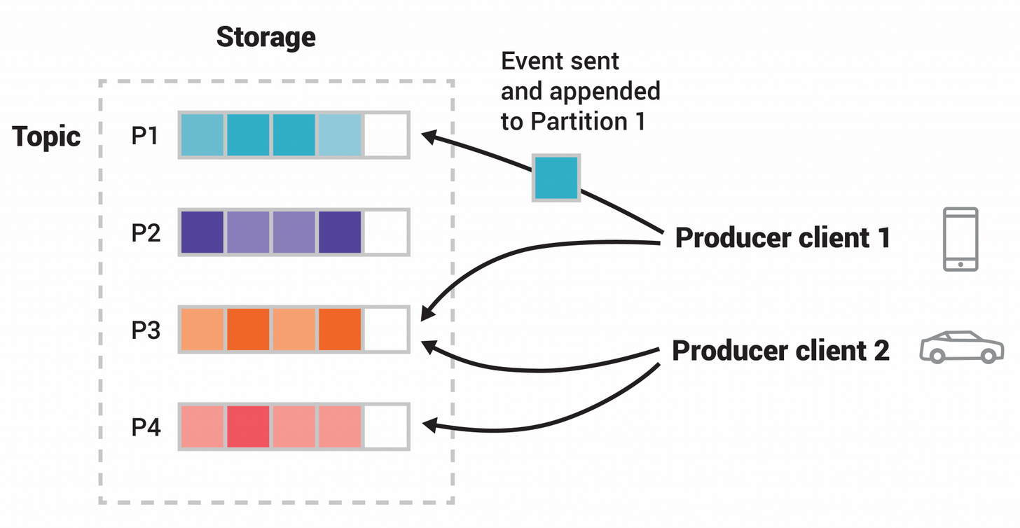
# producers → Kafka topics
# consumers → Kafka topics
# create topic
kafka-topics.sh --create -t events
# producer
kafka-console-producer.sh -t events
# consumer
kafka-console-consumer.sh -t events
# produce events via Kafka
# consume events from Kafka
A city wants to track traffic flow in real time to adjust signals, while also keeping historical data for planning future road expansions.
Would you choose a Data Lake, a Data Warehouse, a Lakehouse, or a Streaming Pipeline?

Realtime data processing enables immediate responses. Events are captured, streamed, and acted upon in seconds, supporting use cases like fraud detection, traffic signals, and IoT monitoring.

MERGE (:Field {id:'A12', name:'North'})
MERGE (:Sensor {id:'S-001', type:'soil'});➜ Created/Found:
Field A12, Sensor S-001MATCH (f:Field {id:'A12'})
MATCH (s:Sensor {id:'S-001'})
MERGE (s)-[:LOCATED_IN]->(f)
RETURN f.id AS field, s.id AS sensor;➜ field | sensor
A12 | S-001MATCH (s:Sensor {id:'S-001'})
CREATE (r:Reading {
at: datetime(), moisture:14
})-[:FROM]->(s)
RETURN s.id AS sensor, r.moisture AS m;➜ sensor | m
S-001 | 14MATCH (f:Field {id:'A12'})<-[:LOCATED_IN]-
(s:Sensor)<-[:FROM]-(r:Reading)
WITH s, r
ORDER BY r.at DESC
WITH s, collect(r)[0] AS last
RETURN s.id AS sensor, last.moisture AS m;➜ sensor | m
S-001 | 14MATCH (f:Field)<-[:LOCATED_IN]-(s:Sensor)
MATCH (r:Reading)-[:FROM]->(s)
WITH f.id AS field, avg(r.moisture) AS avg_m
RETURN field, round(avg_m,1) AS avg_m
ORDER BY avg_m ASC;➜ field | avg_m
A12 | 14.0# Repo
git clone https://github.com/SE4CPS/2025-COMP-263.git
cd 2025-COMP-263/labs/lab3
# Install
npm init -y
npm install dotenv neo4j-driver mongodb
# Env
cp .env.template .env # do NOT commit
# Run
node labs/lab3/sampleNeo4jConnection.js
# Expected
Connected to Neo4j Aura!
# Check if error
# - URI / USER / PASSWORD in .env
# - Internet/TLS reachable
// Read & visualize nodes and edges
MATCH (n)-[r]->(m)
RETURN n,r,m
LIMIT 25;
# Run
node labs/lab3/pushNeo4jToMongo.js
# Expected log
Inserted X docs into Mongo lake
# Tip
# If auth fails, check .env connection
Project1.lake// All docs
db.lake.find({})
// Only Neo4j-sourced
db.lake.find({ sourceDB: "Neo4j" })
# Submit: code + screenshots

Sources & Symptoms in Modern Data Pipelines
| Symptom | Likely Cause |
|---|---|
| High latency | I/O wait or serialization |
| Low throughput | Network or CPU bottleneck |
| Queue build-up | Backpressure not handled |
Metrics, Tradeoffs, and Tuning Principles

| Goal | Possible Tradeoff |
|---|---|
| Increase throughput | Higher latency from batching |
| Reduce latency | Less batching → CPU overhead |
| Parallelize tasks | Coordination cost ↑ |
Example: Smart irrigation with 500+ sensors
// Core loop
client.set(sensorId, JSON.stringify({
moisture: 34.8,
temp: 21.7,
ts: Date.now()
}));
// Windowed latency check
avg = sum(latencies) / latencies.length;
console.log(`avg latency ${avg.toFixed(1)} ms`);
// sample Redis data
{
"sensor:field12": {
"moisture": 34.8,
"temp": 21.7,
"ts": 1738893421312
}
}
Fastest server-side database for real-time data
$ redis-server
$ redis-cli ping
PONG
session:usr123api:key:weather-service
// Example: agriculture sensor data
{
"sensor:field12": {
"moisture": 34.8,
"temperature": 21.7,
"timestamp": 1738893421312
}
}
// Session key
"session:usr123" : {
"token": "eyJhbGciOiJIUzI1NiIs...",
"expires": 1738893999000
}
// API request count
"api:weather:getCount" : 4821
// Cache entry
"cache:forecast:stockton" : {
"temp": 21.7,
"humidity": 65,
"ts": 1738893480000
}

SET crop:12 34.8
GET crop:12
# "34.8"
Single value per key, atomic increment/decrement
SET temp:field3 21.5
INCRBYFLOAT temp:field3 0.3
GET temp:field3
# 21.8
Push and pop like a queue or log
LPUSH sensor:log 34.1
LPUSH sensor:log 34.5
LRANGE sensor:log 0 -1
# ["34.5","34.1"]
Mini key-value maps (like JSON objects)
HSET field:12 moisture 34.8 temp 21.7
HGETALL field:12
HGET field:12 temp
# moisture:34.8, temp:21.7
Unordered unique elements
SADD crops wheat barley maize
SMEMBERS crops
# wheat barley maize
Scores + values → leaderboards or metrics
ZADD soil_moisture 34.8 field12 35.4 field13
ZRANGE soil_moisture 0 -1 WITHSCORES
Append-only logs for real-time pipelines
XADD sensor:stream * moisture 34.8 temp 21.7
XRANGE sensor:stream - +
TTL = Time-To-Live (measured in seconds)
SET weather:now 21.7 EX 60
TTL weather:now
# 60 (seconds remaining)
# ...after a few seconds...
# 57
# -2 (means key expired)
Real-time messaging between clients
SUBSCRIBE irrigation
PUBLISH irrigation "Start pump A"
| Property | Redis Support |
|---|---|
| Atomicity | Yes (single command) |
| Consistency | Eventual, not strict |
| Isolation | Transactions via MULTI/EXEC |
| Durability | No (by default) |
| DB | Model | Speed | Use Case |
|---|---|---|---|
| Redis | Key-Value | ★★★★★ | Caching / Realtime |
| IndexedDB | Client KV | ★★★☆☆ | Browser storage |
| MongoDB | Document | ★★★☆☆ | Flexible schema |
| SQL | Relational | ★★☆☆☆ | Transactional data |
| Neo4j | Graph | ★★☆☆☆ | Relationships |
A city wants to track traffic flow in real time to adjust signals, while also keeping historical data for planning future road expansions.
Would you choose a Data Lake, a Data Warehouse, a Lakehouse, or a Streaming Pipeline?
npm i express mongodb ioredis dotenv
# .env (example)
PORT=3000
MONGO_HOST=mongodb+srv://cluster0.lixbqmp.mongodb.net
MONGO_USER=comp263_2025
MONGO_PASS=***yourpass***
REDIS_URL=redis://localhost:6379
CACHE_TTL_SECONDS=60
Keep secrets in .env. Don’t commit.
mongodb official driverioredis robust Redis clientLab2.Agriculture and validates env.
authestimatedDocumentCount() on boot for sanity
const client = new MongoClient(`${HOST}/...`, {
useNewUrlParser: true, useUnifiedTopology: true,
auth: { username: USER, password: PASS }, authSource: "admin"
});const Redis = require("ioredis");
const redis = new Redis(process.env.REDIS_URL);
// Optional: redis.on("connect", ...) for logging
SETEX/EX TTL for freshness{ source, timeMs, count, data }X-Response-Time headerfunction withTimer(handler) {
return async (req, res) => {
const t0 = process.hrtime.bigint();
try { await handler(req, res, t0); }
catch (e) { res.status(500).json({ error: String(e) }); }
};
}
function elapsedMs(t0) {
return Number((process.hrtime.bigint() - t0) / 1000000n);
}app.get("/agriculture/mongo", withTimer(async (req, res, t0) => {
const docs = await collection.find({}).limit(500).toArray();
const body = {
source: "mongo", timeMs: elapsedMs(t0),
count: docs.length, data: docs
};
res.set("X-Response-Time", body.timeMs + "ms").json(body);
}));app.get("/agriculture/redis", withTimer(async (req, res, t0) => {
const key = "agri:all:limit500";
const ttl = Number(process.env.CACHE_TTL_SECONDS || 60);
const cached = await redis.get(key);
if (cached) {
const data = JSON.parse(cached);
const body = {
source: "redis", timeMs: elapsedMs(t0),
count: data.length, data
};
return res.set("X-Response-Time", body.timeMs + "ms").json(body);
}
const docs = await collection.find({}).limit(500).toArray();
await redis.set(key, JSON.stringify(docs), "EX", ttl);
const body = {
source: "mongo→redis(set)", timeMs: elapsedMs(t0),
count: docs.length, data: docs
};
res.set("X-Response-Time", body.timeMs + "ms").json(body);
}));# Quick manual check (shows X-Response-Time)
curl -i http://localhost:3000/agriculture/mongo | head
curl -i http://localhost:3000/agriculture/redis | head
curl -i http://localhost:3000/agriculture/redis | head # 2nd# 1. Install Ubuntu on Windows
wsl --install -d Ubuntu
# Restart when prompted, then open Ubuntu
# 2. Inside Ubuntu
sudo apt update
sudo apt install -y redis-server
sudo service redis-server start
redis-cli ping # → PONG
REDIS_URL=redis://127.0.0.1:6379 in .envbrew update
brew install redis
brew services start redis
redis-cli ping # → PONG
brew services127.0.0.1:6379Approximate time to retrieve one object at different data scales.
| Dataset Size | Redis (In-Memory) | MongoDB (Disk-Based) | Relative Speed |
|---|---|---|---|
| 1 record | ~1 ms | ~100 ms | ≈ 100× faster |
| 1,000 records | ~2 ms | ~120 ms | ≈ 60× faster |
| 100,000 records | ~5 ms | ~250 ms | ≈ 50× faster |
| 1,000,000 records | ~10 ms | ~600 ms | ≈ 60× faster |
SET key value stores a string value.GET key retrieves it.const Redis = require("ioredis");
const redis = new Redis();
// Store data
await redis.set("crop:rice", JSON.stringify({ yield: 45 }));
// Retrieve data
const value = await redis.get("crop:rice");
console.log(JSON.parse(value));SETEX key ttl valueredis.set(key, value, "EX", ttl)await redis.set("weather:stockton",
JSON.stringify({ temp: 29 }),
"EX", 60); // expires in 60 seconds
const cached = await redis.get("weather:stockton");
console.log(cached ? "Cache hit" : "Expired");DEL key removes one or more keys.EXISTS key checks if a key is present.await redis.del("weather:stockton");
const exists = await redis.exists("weather:stockton");
if (exists) console.log("Still cached");
else console.log("Cache cleared or expired");TTL key shows remaining lifetime (in seconds).EXPIRE key seconds sets a new TTL for an existing key.await redis.set("session:123", "active");
await redis.expire("session:123", 120);
const ttl = await redis.ttl("session:123");
console.log("Time left:", ttl, "seconds");MSET sets multiple keys at once.MGET retrieves multiple keys in one call.await redis.mset({
"crop:wheat": "good",
"crop:rice": "medium",
"crop:corn": "low"
});
const values = await redis.mget(
"crop:wheat",
"crop:rice",
"crop:corn"
);
console.log(values);FLUSHDB removes all keys from the current database.KEYS pattern lists keys matching a pattern.const allKeys = await redis.keys("crop:*");
console.log("Found:", allKeys.length, "keys");
await redis.flushdb(); // clears all keys in this DB
console.log("Database cleared");
graph LR
A[Client Request] --> B[Check Cache]
B -->|Hit| C[Return from Cache]
B -->|Miss| D[Fetch from DB]
D --> E[Update Cache]
E --> F[Return to Client]
graph LR
A[Client Write] --> B[Update Cache]
B --> C[Write to DB]
C --> D[Success Response]
flowchart LR A["Client Write"] --> B["Write to Cache"] B --> C["Async Queue"] C --> D["DB Update (Delayed)"]
graph LR
A[Client Request] --> B[Cache Layer]
B -->|Hit| C[Return from Cache]
B -->|Miss| D[Cache Loads from DB]
D --> E[Store in Cache & Return]
graph TD
A[Data Stored] --> B[Timer Starts]
B -->|TTL Expires| C[Auto Delete]
C --> D[Cache Miss Next Time]
D --> E[Reload from DB]
Sample Midterm
Answers
Which “V” primarily addresses the challenge of many formats (logs, images, JSON) in one system?
Answer: B: Variety
Why must IndexedDB operations be awaited in JavaScript?
Answer: C: Asynchronous I/O (Promise)
What is automatically indexed in an IndexedDB object store?
Answer: A: Primary key
Which choice best explains why rigid SQL schemas struggle with fast-changing app fields?
Answer: D: Migrations required
Which practice improves read performance for common UI queries in document models?
Answer: C: Denormalize frequent fields
Which identifier minimizes cross-system collisions without coordination?
Answer: B: UUID v4
What does the “Z” in 2025-09-04T10:15:30Z denote?
Answer: A: UTC
When is embedding (not reference) generally preferred in JSON document design?
Answer: D: Always fetched together
Which metric ensures each real-world entity appears only once?
Answer: B: Uniqueness
What is the primary benefit of a UNIQUE index on a field such as email?
Answer: A: Prevent duplicates
A dataset missing required fields most directly violates which quality dimension?
Answer: D: Completeness
Stale sensor values mainly reduce which property?
Answer: C: Timeliness
In ELT, where is heavy transformation primarily performed?
Answer: A: In the target store
Which workload fits streaming best?
Answer: D: IoT telemetry
In MapReduce, which phase combines intermediate key groups into final values?
Answer: B: Reduce
Which choice improves throughput for many small writes?
Answer: C: Batch operations
Which property distinguishes a data lake from a warehouse?
Answer: B: Schema-on-read
Where are raw, unprocessed files usually stored before cleaning and structuring?
Answer: B: In the initial lake for incoming data data
Which query pattern is a strength of a graph database?
Answer: A: Multi-hop traversal
Which component most directly decouples producers and consumers?
Answer: C: Broker/Queue
Which design is typical for an analytical warehouse model?
Answer: D: Star/Snowflake
How do relational databases typically support aggregation such as SUM or AVG?
Answer: C: SQL aggregate functions in the query engine
What is the main goal of moving data from a data lake into a data warehouse?
Answer: B: Organize data for analytics
During transformation from data lake to data warehouse, which step typically occurs?
Answer: C: Clean, join, and aggregate curated data
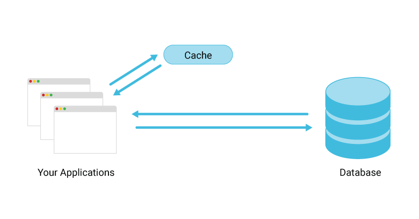
In cache-aside, what happens on a cache miss?
Answer: B: Load DB → populate cache → return
Which Redis option sets expiration when writing a value?
SET ... NXSET ... PXAT onlyPERSISTSET key value EX <seconds>Answer: D: SET ... EX <seconds>
What best measures API latency difference between Mongo and Redis endpoints?
timeMs & X-Response-Time)Answer: A: Server-side timing
Which practice balances speed and freshness for frequently changing data?
Answer: C: Short TTL + cache-aside
yield values?harvest_date in valid ISO format?region names?yield?farm_id?
{
"farm_id": "F123",
"crop": "rice",
"region": "California",
"yield": "72 tons",
"soil": {
"type": "clay",
"ph": 9.8
},
"harvest_date": "10-09-25"
}

{
"metric": "rainfall",
"value": 8,
"unit": "mm",
"timestamp_utc": "2025-10-21T00:00:00Z"
}
{
"kpi": "weekly_rainfall",
"average_value": 42,
"unit": "mm/week",
"week_start_utc": "2025-10-20T00:00:00Z",
"data_points": 7
}
{
"target": "weekly_rainfall",
"goal_value": 40,
"unit": "mm/week",
"valid_from_utc": "2025-10-01T00:00:00Z",
"valid_to_utc": "2025-12-31T23:59:59Z"
}
{
"benchmark": "weekly_rainfall_by_crop",
"crops": {
"corn": 40,
"wheat": 30,
"soybean": 35
},
"unit": "mm/week",
"reference_period": "2024",
"source": "historical_weather_data"
}
| Relationship | Description | Example |
|---|---|---|
| Metric → KPI | Daily rainfall readings combine to calculate weekly averages. | {"rainfall_daily":[8,5,6,7,10,4,2]} |
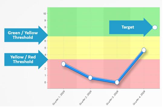
| KPI ↔ Benchmark | Compare weekly rainfall KPI to historical averages by crop type. | Corn = 40 mm, Wheat = 30 mm, Soybean = 35 mm |
| KPI → Target | If the KPI is below the 40 mm target, schedule additional irrigation. | Current = 32 mm → Add irrigation |
| Loop | Metrics feed into KPI → compared to benchmark → adjusted toward target. | Continuous weekly update and correction cycle |
{
"rainfall_daily": [8, 5, 6, 7, 10, 4, 2],
"min": 2,
"max": 10,
"sum": 42,
"avg": 6.0
}
CREATE TABLE example_types
(
id UInt32,
name String,
score Float64,
tags Array(String),
metrics Map(String, Float32),
status Enum8('ok'=1, 'fail'=2),
created_at DateTime64(3),
uid UUID,
extra Nullable(String)
)
ENGINE = MergeTree();
-- ClickHouse adds Array, Tuple, Map, Enum, LowCardinality, Nested, UUID
SELECT user_id, ts, duration
FROM logs
WHERE event = 'page_view'
LIMIT 3;
┌─user_id─┬────────ts────────┬─duration─┐
│ 101 │ 2025-10-23 10:00 │ 120 │
│ 102 │ 2025-10-23 09:59 │ 95 │
│ 103 │ 2025-10-23 09:58 │ 134 │
└─────────┴──────────────────┴──────────┘
SELECT url, count() AS views, avg(duration) AS avg_ms
FROM logs
GROUP BY url
ORDER BY views DESC
LIMIT 3;
┌─url──────────────┬─views─┬─avg_ms─┐
│ /home │ 12500 │ 112.4 │
│ /products │ 9432 │ 98.3 │
│ /checkout │ 2831 │ 145.6 │
└──────────────────┴───────┴────────┘
SELECT user_id, action
FROM user_activity
ARRAY JOIN actions AS action
LIMIT 3;
┌─user_id─┬─action───┐
│ 101 │ click │
│ 101 │ scroll │
│ 102 │ view │
└─────────┴──────────┘
SELECT
user_id,
ts,
avg(duration) OVER (
PARTITION BY user_id
ORDER BY ts
ROWS BETWEEN 4 PRECEDING AND CURRENT ROW
) AS avg_last_5
FROM sessions
LIMIT 3;
┌─user_id─┬────────ts────────┬─avg_last_5─┐
│ 101 │ 2025-10-23 10:00 │ 98.4 │
│ 101 │ 2025-10-23 10:05 │ 102.7 │
│ 101 │ 2025-10-23 10:10 │ 95.8 │
└─────────┴──────────────────┴────────────┘
INSERT INTO logs (ts, user_id, event, duration)
VALUES (now(), 101, 'view', 120),
(now(), 102, 'click', 85);
Query OK, 2 rows inserted.
Elapsed: 0.002 sec.
SELECT query_kind, read_rows, memory_usage
FROM system.query_log
LIMIT 2;
┌─query_kind─┬─read_rows─┬─memory_usage─┐
│ Select │ 21000 │ 15.2 MiB │
│ Insert │ 2000 │ 2.8 MiB │
└────────────┴────────────┴──────────────┘
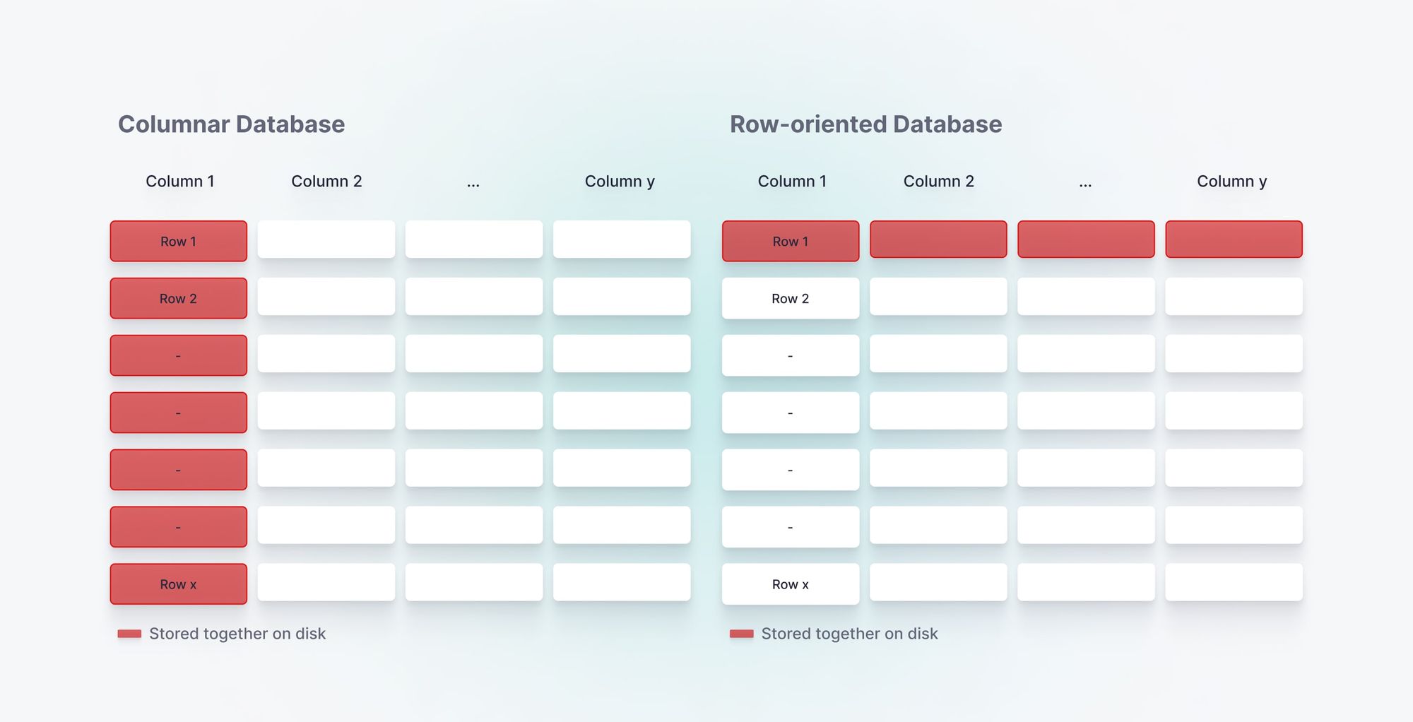

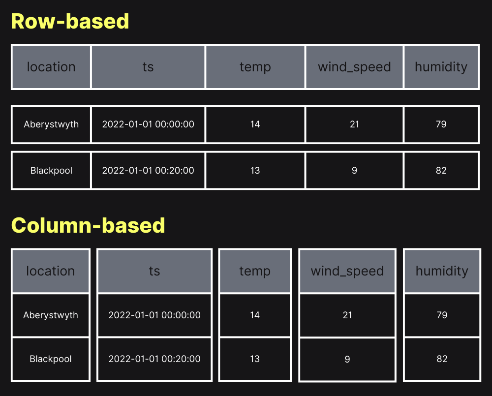
| Query Type | Use Row-Based DB | Use Column-Based DB |
|---|---|---|
| Inserts and Updates | ✔ | |
| Single-row lookups | ✔ | |
| Aggregations over large datasets | ✔ | |
| Reporting and analytics | ✔ | |
| Real-time dashboards | ✔ |
| Use Columnar Databases When... | Use Row-Oriented Databases When... |
|---|---|
| Your primary use case is analytics | Your primary use case is transactions |
| You need low query latency for large scans | You don't need low latency for analytics |
| You have large amounts of analytical data | You're working with smaller data sets |
| You don't need strict ACID compliance | You need strict ACID compliance |
| You're using event sourcing principles | You perform frequent, small updates or deletes |
| You store and analyze time series data | You access records by unique IDs |
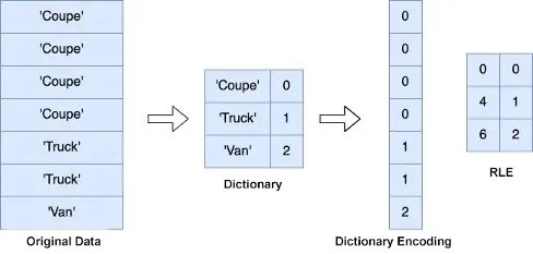
| Storage Type | Aggregation Time Complexity | Reason |
|---|---|---|
| Row-Based | O(n × m) | Scans all rows and all columns |
| Column-Based | O(n) | Scans only the relevant column |
n = number of rows, m = number of columns
| Concept | Column-Based DB | Row-Based DB |
|---|---|---|
| Data Layout | Columns stored independently | Rows stored together |
| Indexing Need | Often reduced due to scan efficiency | Critical for performance |
| Default Access | Column filters without indexes are fast | Needs indexes for efficient filtering |
| Index Type | Skip indexes, min-max indexes, sparse indexes | B-tree, hash, GIN, GiST |
| Compression & Filtering | Efficient filtering via compressed column blocks | Filtering depends on explicit indexes |
| Example | ClickHouse: Primary index is skip-based by default | PostgreSQL: Uses B-tree indexes by default |
| Feature | ClickHouse | PostgreSQL |
|---|---|---|
| Storage Model | Column-based | Row-based |
| Primary Use Case | Analytics (OLAP) | Transactions (OLTP) |
| Indexing | Skip index (min-max, sparse) | B-tree, hash, GIN, GiST |
| Write Performance | High-throughput batch inserts | Optimized for single-row inserts |
| Read Performance | Fast scans on large datasets | Fast lookups and joins |
| Compression | Built-in, column-aware compression | Optional extensions |
| SQL Support | Subset of ANSI SQL (e.g., no FULL OUTER JOIN, no foreign keys) | Full ANSI SQL with rich extensions |
| ACID Compliance | Eventual consistency, no full ACID | Full ACID compliance |
| Description | SQL Query |
|---|---|
| Average trip distance |
|
| Average fare amount |
|
| Average tip by payment type |
|
| Average total amount by vendor |
|
A vineyard in California struggled with soil moisture variations, risking crop quality. The benchmark from state guidelines required maintaining 25–35% moisture.
The farm set a target of keeping soil moisture near 30% using IoT-based irrigation control.
The main KPI was average soil moisture per zone, updated hourly through a data pipeline.
Supporting metrics included pump runtime, water flow rate, and daily irrigation volume. Within weeks, dashboard insights cut water use by 15% while staying within target range.
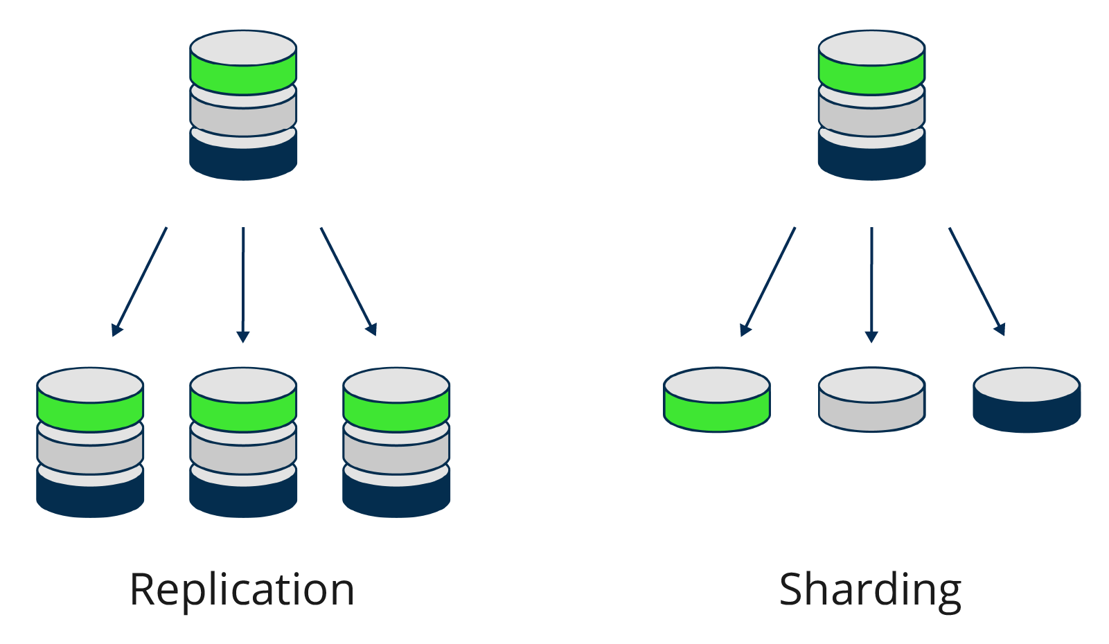
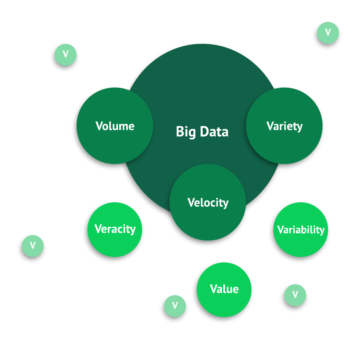
Adding more machines or nodes to a system to increase capacity and distribute load.
Increasing the capacity of an existing machine by adding more resources such as CPU or RAM.
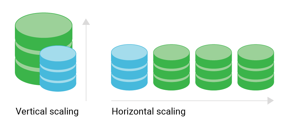
Distributed Databases lead to the CAP Theorem balancing Consistency, Availability, and Partition Tolerance.
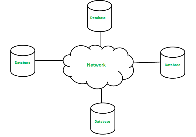
Under a partition, you can favor C or A, not both.
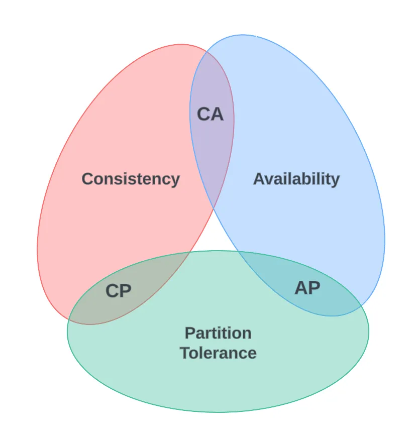
Together, they improve scalability, availability, and resilience of large systems.

| Database | Consistency + Partition Tolerance (CP) | Consistency + Availability (CA) | Availability + Partition Tolerance (AP) |
|---|---|---|---|
| MongoDB/Redis | ✔ | ✘ | ✘ |
| Cassandra | ✘ | ✘ | ✔ |
| RDBMS | ✘ | ✔ | ✘ |
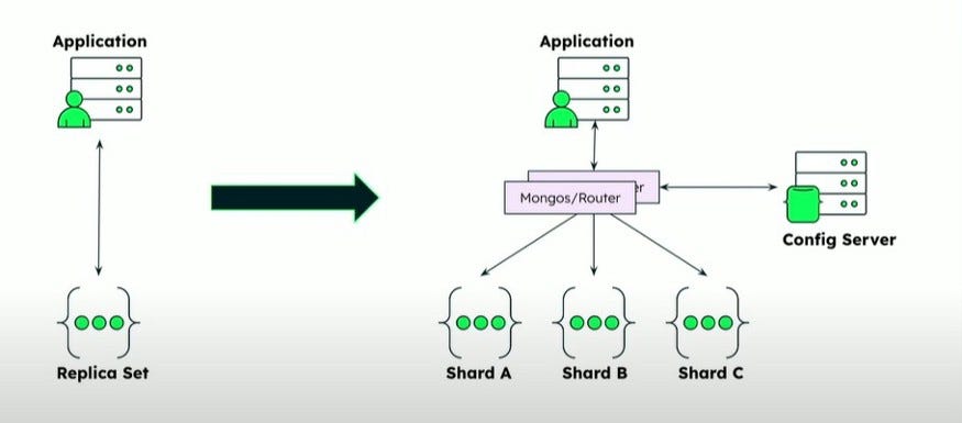
| Aspect | Replica Set | Shard |
|---|---|---|
| Purpose | Provides redundancy and failover. | Distributes data for scalability. |
| Data Stored | Same crop data copied across nodes. | Different crop regions stored on different shards. |
| Example | All nodes store “Wheat yield 2024” dataset. | Shard A = Wheat (North farms), Shard B = Corn (South farms). |
| Goal | Reliability and availability. | Scalability and performance. |
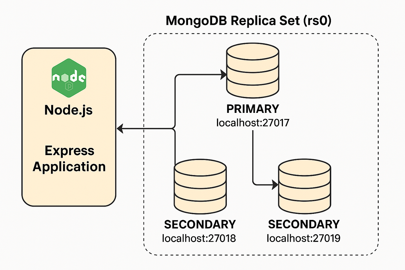
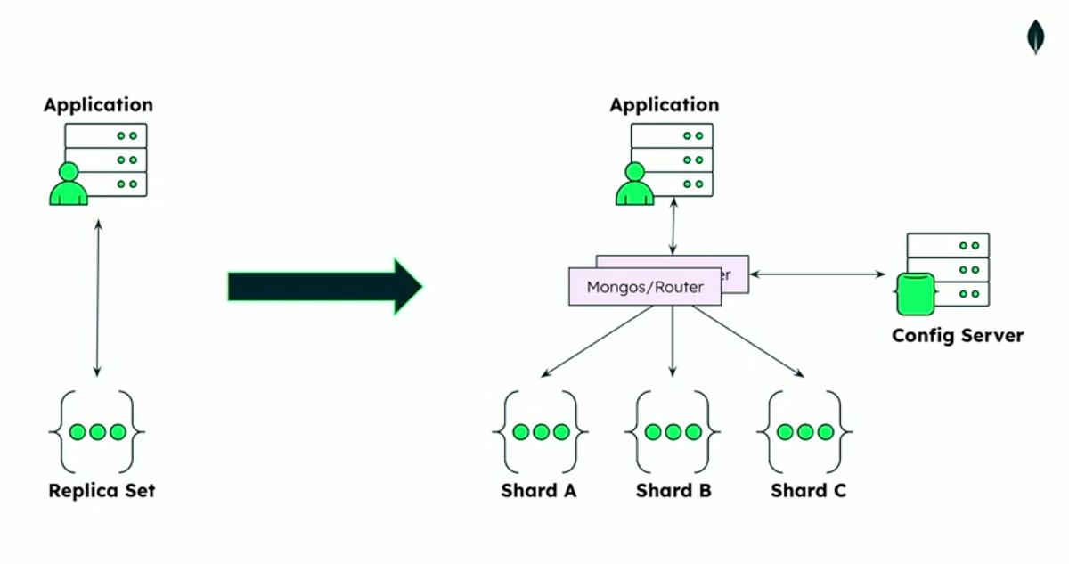

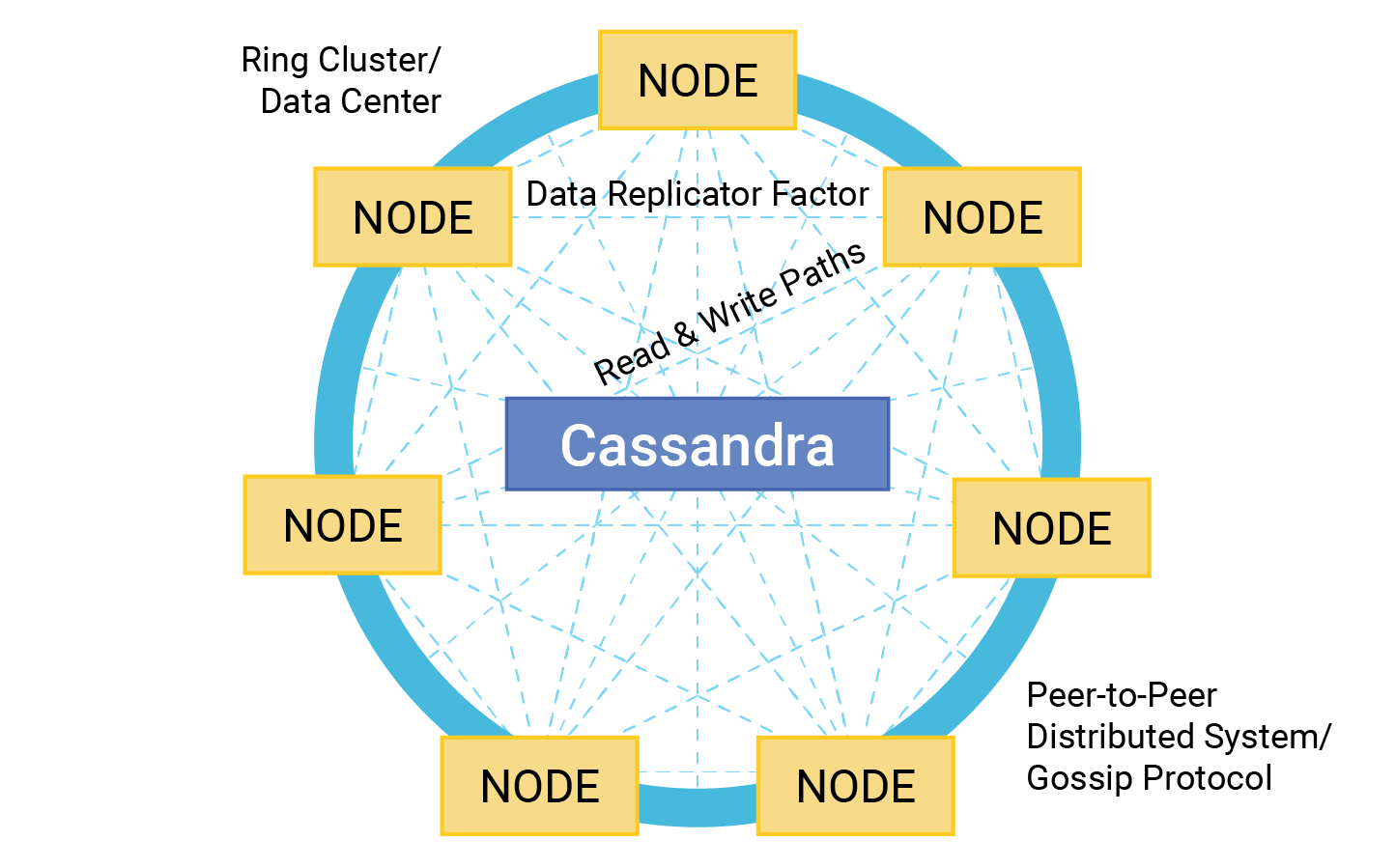
Keeps cluster consistent and fault-aware.

CREATE KEYSPACE farm_data
WITH REPLICATION = {'class':'SimpleStrategy', 'replication_factor':3};
CREATE TABLE crop_yields (
farm_id text,
crop_type text,
year int,
yield double,
PRIMARY KEY ((farm_id), crop_type, year)
);
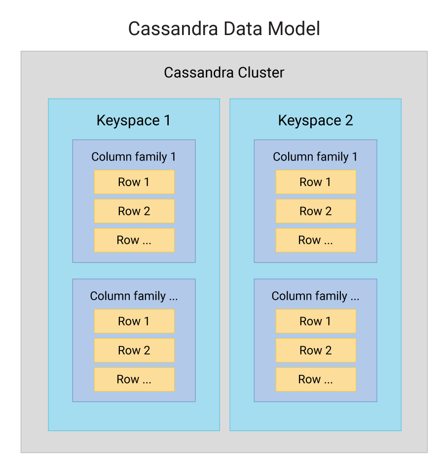
Coordinator enforces consistency across replicas
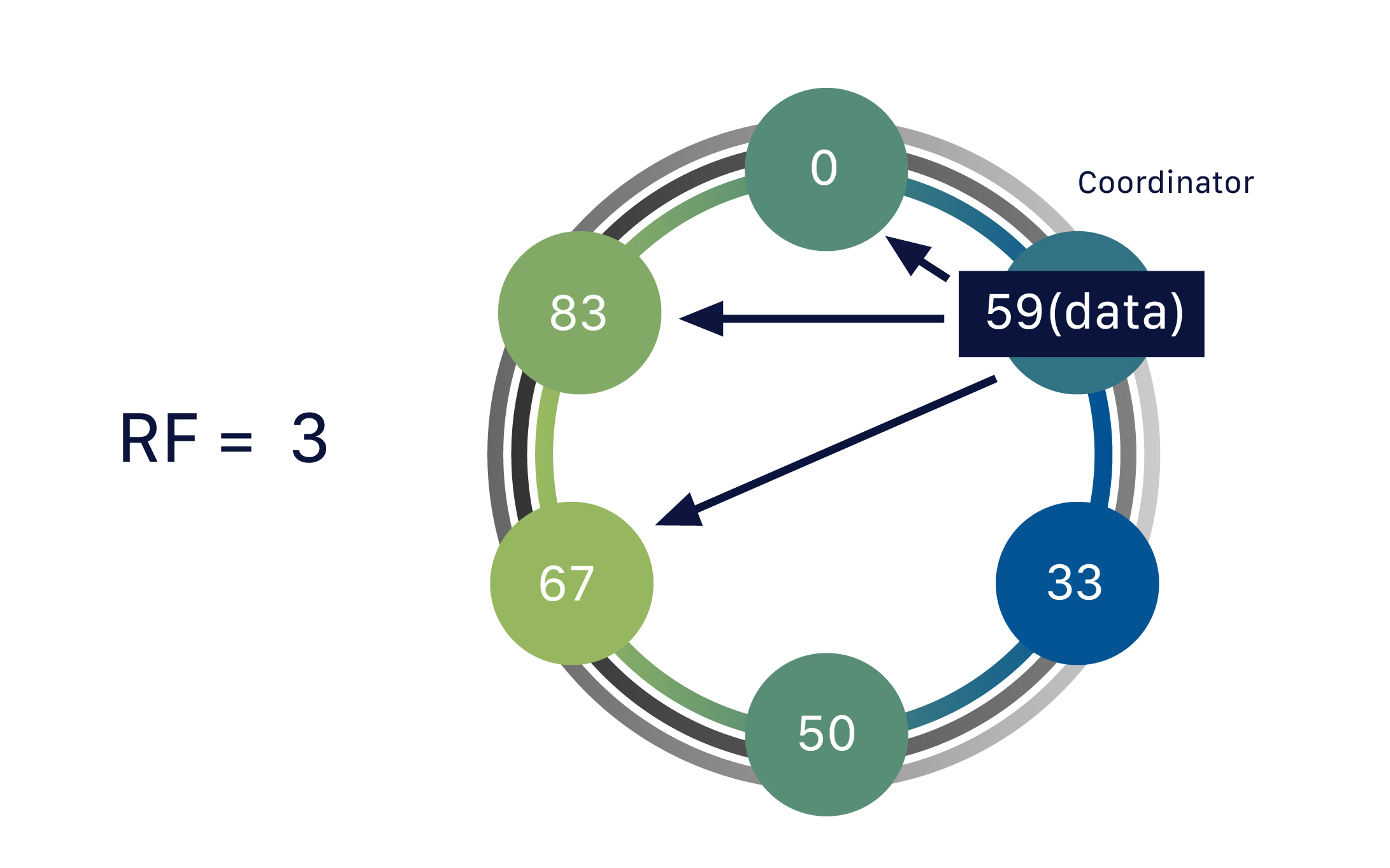
→ Cassandra is AP (Availability + Partition Tolerance)
CREATE TABLE sensor_data (
farm_id text,
sensor_id text,
ts timestamp,
temp float,
moisture float,
PRIMARY KEY ((farm_id, sensor_id), ts)
) WITH CLUSTERING ORDER BY (ts DESC);

(farm_id)(sensor_id, ts)
CREATE TABLE sensor_data (
farm_id text,
sensor_id text,
ts timestamp,
value float,
PRIMARY KEY ((farm_id), sensor_id, ts)
);
Partition Key: farm_id → decides node placement
Clustering Keys: sensor_id, ts → order within partition
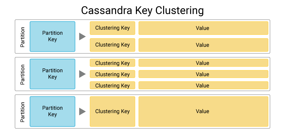
| Pipeline Stage | Data Type / Need | Best Database | Reason |
|---|---|---|---|
| Sensor Ingestion | High-volume IoT readings (temperature, soil, humidity) | ? | Handles fast writes, distributed and fault-tolerant |
| Short-term Analytics | Recent sensor trends (last 24h) | ? | Flexible schema, easy aggregation pipelines |
| Long-term Storage | Historical yields and weather data | ? | Supports structured queries and analytics |
| Real-time Alerts | Threshold-based triggers (low moisture) | ? | In-memory, fast pub/sub messaging |
| Visualization & Dashboards | Aggregated farm metrics and KPIs | ? | Optimized for analytics and fast group-by queries |

-- SQL
SELECT f.id, f.name, h.crop, h.yield_kg
FROM farmers f
JOIN harvest_lots h ON h.farmer_id = f.id
WHERE f.id = 42;
-- MQL
db.farmers.find(
{ _id: 42 },
{ name: 1, harvestLots: 1 }
);
{
"_id": 42,
"name": "Alice Farms",
"harvestLots": [
{ "crop": "Wheat", "yieldKg": 18000 },
{ "crop": "Corn", "yieldKg": 24500 }
]
}
-- SQL
INSERT INTO soil_events(sensor_id, ts, moisture, temp)
VALUES (17, NOW(), 23.4, 21.7);
-- MQL
db.soilSensors.updateOne(
{ _id: "sensor-17" },
{ $push: { readings: { ts: ISODate(), moisture: 23.4 } } },
{ upsert: true }
);
{
"_id": "sensor-17",
"readings": [
{ "ts": "2025-11-05T04:00:00Z", "moisture": 23.4 }
]
}
-- SQL
ALTER TABLE crops ADD COLUMN agronomy_json JSON;
-- MQL
db.crops.insertOne({
_id: "crop-123",
name: "Tomato",
agronomy: { variety: "Roma", irrigation: "drip" },
inputs: [{ name: "NPK-10-10-10", rateKgPerHa: 120 }]
});
{
"_id": "crop-123",
"name": "Tomato",
"agronomy": { "variety": "Roma", "irrigation": "drip" },
"inputs": [{ "name": "NPK-10-10-10", "rateKgPerHa": 120 }]
}
-- SQL
INSERT INTO yield_clean
SELECT * FROM yield_stage WHERE valid = TRUE;
-- MQL
db.yieldReports.insertOne({
_id: "YR-7",
fieldId: "F-101",
raw: { yieldKg: "??", moisture: "N/A", source: "c_csv" },
clean: { yieldKg: 17450, moisture: 13.2 },
quality: { valid: false, issues: ["missing_yield"] },
lineage: { file: "coop_2025-11-05.csv" }
});
{
"_id": "YR-7",
"fieldId": "F-101",
"raw": { "yieldKg": "??", "moisture": "N/A", "source": "c_csv" },
"clean": { "yieldKg": 17450, "moisture": 13.2 },
"quality": { "valid": false, "issues": ["missing_yield"] },
"lineage": { "file": "coop_2025-11-05.csv" }
}
-- SQL
SELECT * FROM farmers WHERE id=42;
SELECT SUM(yield_kg)
FROM harvest_lots WHERE farmer_id=42;
-- MQL
db.farmers.find(
{ _id: 42 },
{ name: 1, harvestLots: 1, metrics: 1 }
);
{
"_id": 42,
"name": "Alice Farms",
"harvestLots": [
{ "crop": "Wheat", "yieldKg": 18000 },
{ "crop": "Corn", "yieldKg": 24500 }
],
"metrics": { "totalYieldKg": 42500, "lastHarvestId": 902 }
}

{
"_id": "...",
"farmerName": "...",
"fields": [
{
"fieldId": "...",
"crop": {
"name": "...",
"variety": "...",
"agronomy": {
"irrigation": "...",
"spacingCm": ...
}
},
"sensors": [
{
"sensorId": "...",
"type": "...",
"readings": [
{ "ts": "...", "moisture": ..., "temp": ... },
...
]-- 1:1
{
"_id": "farmer-101",
"profile": { "name": "Alice", "address": "..." }
}
-- 1:N
{
"_id": "field-22",
"crop": "Wheat",
"harvestLots": [
{ "lotId": "L-1", "yieldKg": 18000 },
{ "lotId": "L-2", "yieldKg": 24500 }
]
}
-- N:N (using references)
{
"_id": "coop-7",
"name": "Central Farm Cooperative",
"farmers": [
{ "$ref": "farmers", "$id": "farmer-101" },
{ "$ref": "farmers", "$id": "farmer-102" }
],
"equipment": [
{ "$ref": "equipment", "$id": "tractor-55" },
{ "$ref": "equipment", "$id": "harvester-21" }
]
}

farmer.id = farmer_profile.farmer_id-- SQL tables
farmers
├─ id
├─ name
└─ region
farmer_profile
├─ farmer_id (FK)
├─ address
└─ contact_number
{
"_id": "farmer-101",
"name": "Alice Farms",
"region": "Central Valley",
"profile": {
"address": "...",
"contactNumber": "...",
"farmSizeHectares": ...,
"certifications": ["Organic", "Sustainable"]
}
}
// SQL source rows
const farmers = [
{ id: 1, name: "Alice Farms", region: "Central" },
{ id: 2, name: "Bob Fields", region: "South" }
];
const profiles = [
{ farmer_id: 1, address: "...", contact: "...", size_ha: 12 },
{ farmer_id: 2, address: "...", contact: "...", size_ha: 9 }
];
// Transformation
const merged = farmers
.map(f => {
const profile = profiles.find(p => p.farmer_id === f.id);
return { ...f, profile };
})
.filter(d => d.profile) // ensure valid links
.reduce((acc, doc) => [...acc, doc], []);
// Result → JSON documents
console.log(JSON.stringify(merged, null, 2));
[
{
"_id": 1,
"name": "Alice Farms",
"region": "Central",
"profile": {
"address": "...",
"contact": "...",
"sizeHa": 12
}
},
{
"_id": 2,
"name": "Bob Fields",
"region": "South",
"profile": {
"address": "...",
"contact": "...",
"sizeHa": 9
}
}
]
harvest_lots.farmer_id → farmers.id-- SQL tables
farmers
├─ id
├─ name
└─ region
harvest_lots
├─ id
├─ farmer_id (FK)
├─ crop
└─ yield_kg
{
"_id": "farmer-101",
"name": "Alice Farms",
"region": "Central Valley",
"harvestLots": [
{ "lotId": "L-1", "crop": "Wheat", "yieldKg": 18000 },
{ "lotId": "L-2", "crop": "Corn", "yieldKg": 24500 }
]
}
harvestLots array// SQL source rows
const farmers = [
{ id: 1, name: "Alice Farms", region: "Central" },
];
const harvestLots = [
{ id: "L-1", farmer_id: 1, crop: "Wheat", yield_kg: 18000 },
{ id: "L-2", farmer_id: 1, crop: "Corn", yield_kg: 24500 },
];
// Transformation (group lots under each farmer)
const docs = farmers.map(f => {
const lots = harvestLots
.filter(l => l.farmer_id === f.id)
.reduce((acc, l) => [
...acc,
{ lotId: l.id, crop: l.crop, yieldKg: l.yield_kg }
], []);
return { _id: f.id, name: f.name, region: f.region,... };
});
[
{
"_id": 1,
"name": "Alice Farms",
"region": "Central",
"harvestLots": [
{ "lotId": "L-1", "crop": "Wheat", "yieldKg": 18000 },
{ "lotId": "L-2", "crop": "Corn", "yieldKg": 24500 }
]
},
{
"_id": 2,
"name": "Bob Fields",
"region": "South",
"harvestLots": [
{ "lotId": "L-3", "crop": "Tomato", "yieldKg": 9000 }
]
}
]
-- SQL tables
farmers
├─ id
└─ name
equipment
├─ id
└─ type
farmer_equipment
├─ farmer_id (FK → farmers.id)
└─ equipment_id (FK → equipment.id)
{
"_id": "farmer-101",
"name": "Alice Farms",
"equipmentIds": ["tractor-55", "harvester-21"]
}
{
"_id": "tractor-55",
"type": "Tractor",
"farmerIds": ["farmer-101", "farmer-204"]
}
farmerId and equipmentId{
"_id": "link-9001",
"farmerId": "farmer-101",
"equipmentId": "tractor-55",
"since": "..."
}
{
"_id": "link-9002",
"farmerId": "farmer-204",
"equipmentId": "tractor-55",
"since": "..."
}
equipmentIds arrays// SQL source rows
const farmers = [
{ id: 101, name: "Alice Farms" }
];
const equipment = [
{ id: "tractor-55", type: "Tractor" }
];
const farmerEquipment = [
{ farmer_id: 101, equipment_id: "tractor-55" },
{ farmer_id: 101, equipment_id: "harvester-21" }
];
// Build reference arrays on farmer docs
const farmerDocs = farmers.map(f => {
const eqIds = farmerEquipment
.filter(link => link.farmer_id === f.id)
.reduce((acc, link) => [...acc, link.equipment_id], []);
return { _id: `farmer-${f.id}`, name: f.name, equipIds: eqIds };
});
[
{
"_id": "farmer-101",
"name": "Alice Farms",
"equipmentIds": ["tractor-55", "harvester-21"]
},
{
"_id": "farmer-204",
"name": "Bob Fields",
"equipmentIds": ["tractor-55"]
}
]
farmerEquipmentLinks docs// Build linking collection documents
const farmerEquipmentLinks = farmerEquipment
.map((l, i) => ({
_id: `link-${i + 1}`,
farmerId: `farmer-${l.farmer_id}`,
equipmentId: l.equipment_id,
since: "..."
}))
.filter(link => link) // placeholder for conditions
.reduce((acc, link) => [...acc, link], []);
[
{
"_id": "link-1",
"farmerId": "farmer-101",
"equipmentId": "tractor-55",
"since": "..."
},
{
"_id": "link-2",
"farmerId": "farmer-101",
"equipmentId": "harvester-21",
"since": "..."
},
{
"_id": "link-3",
"farmerId": "farmer-204",
"equipmentId": "tractor-55",
"since": "..."
}
]
Agriculture system tables:
| farmers | id | name | region | |
|---|---|---|---|---|
| farmer_profiles | id | farmer_id | phone | |
| harvest_lots | id | farmer_id | crop | yield_kg |
| buyers | id | name | ||
| contracts | farmer_id | buyer_id |
Reports are slow due to joins.
ETL (Extract → Transform → Load)
SQL → map/filter/reduce → JSONELT (Extract → Load → Transform)
JSON → load → enrich(meta, totals)const farmers=[{id:1,name:"Alem",region:"Delta"},
{ id:2,name:"Maya",region:"Central" }];
const farmer_profiles=[{farmer_id:1,phone:"555-1111"},
{ farmer_id:2,phone:"555-2222" }];
const harvests=[{id:1,farmer_id:1,crop:"Tomato",yield_kg:300},
{ id:2,farmer_id:1,crop:"Onion",yield_kg:200 },
{ id:3,farmer_id:2,crop:"Wheat",yield_kg:500 }];
const buyers=[{id:10,name:"FreshMart"},
{ id:20,name:"AgriCo" }];
const contracts=[{farmer_id:1,buyer_id:10},
{ farmer_id:1,buyer_id:20 },
{ farmer_id:2,buyer_id:10 }];farmers ⟷ farmer_profilesconst farmerDocs_1x1=farmers.map(f=>{
const p=farmer_profiles.find(x=>x.farmer_id===f.id);
return {...f,profile:p};
});farmers ⟷ harvestsconst farmers=[{id:1,name:"Alem",region:"Delta"},
{ id:2,name:"Maya",region:"Central" }];
const farmer_profiles=[{farmer_id:1,phone:"555-1111"},
{ farmer_id:2,phone:"555-2222" }];
const harvests=[{id:1,farmer_id:1,crop:"Tomato",yield_kg:300},
{ id:2,farmer_id:1,crop:"Onion",yield_kg:200 },
{ id:3,farmer_id:2,crop:"Wheat",yield_kg:500 }];
const buyers=[{id:10,name:"FreshMart"},
{ id:20,name:"AgriCo" }];
const contracts=[{farmer_id:1,buyer_id:10},
{ farmer_id:1,buyer_id:20 },
{ farmer_id:2,buyer_id:10 }];const farmerDocs_1xn=farmers.map(f=>({
...f,
harvests:harvests.filter(h=>h.farmer_id===f.id)
}));sum yield_kgconst farmers=[{id:1,name:"Alem",region:"Delta"},
{ id:2,name:"Maya",region:"Central" }];
const farmer_profiles=[{farmer_id:1,phone:"555-1111"},
{ farmer_id:2,phone:"555-2222" }];
const harvests=[{id:1,farmer_id:1,crop:"Tomato",yield_kg:300},
{ id:2,farmer_id:1,crop:"Onion",yield_kg:200 },
{ id:3,farmer_id:2,crop:"Wheat",yield_kg:500 }];
const buyers=[{id:10,name:"FreshMart"},
{ id:20,name:"AgriCo" }];
const contracts=[{farmer_id:1,buyer_id:10},
{ farmer_id:1,buyer_id:20 },
{ farmer_id:2,buyer_id:10 }];const withTotals=farmerDocs_1xn.map(f=>({
...f,
total_yield:f.harvests.reduce((s,h)=>s+h.yield_kg,0)
}));yield_kg >= 300const farmers=[{id:1,name:"Alem",region:"Delta"},
{ id:2,name:"Maya",region:"Central" }];
const farmer_profiles=[{farmer_id:1,phone:"555-1111"},
{ farmer_id:2,phone:"555-2222" }];
const harvests=[{id:1,farmer_id:1,crop:"Tomato",yield_kg:300},
{ id:2,farmer_id:1,crop:"Onion",yield_kg:200 },
{ id:3,farmer_id:2,crop:"Wheat",yield_kg:500 }];
const buyers=[{id:10,name:"FreshMart"},
{ id:20,name:"AgriCo" }];
const contracts=[{farmer_id:1,buyer_id:10},
{ farmer_id:1,buyer_id:20 },
{ farmer_id:2,buyer_id:10 }];const highYield=withTotals.map(f=>({
...f,
harvests:f.harvests.filter(h=>h.yield_kg>=300)
}));farmers ⟷ contracts ⟷ buyersconst farmers=[{id:1,name:"Alem",region:"Delta"},
{ id:2,name:"Maya",region:"Central" }];
const farmer_profiles=[{farmer_id:1,phone:"555-1111"},
{ farmer_id:2,phone:"555-2222" }];
const harvests=[{id:1,farmer_id:1,crop:"Tomato",yield_kg:300},
{ id:2,farmer_id:1,crop:"Onion",yield_kg:200 },
{ id:3,farmer_id:2,crop:"Wheat",yield_kg:500 }];
const buyers=[{id:10,name:"FreshMart"},
{ id:20,name:"AgriCo" }];
const contracts=[{farmer_id:1,buyer_id:10},
{ farmer_id:1,buyer_id:20 },
{ farmer_id:2,buyer_id:10 }];const farmerWithBuyers=farmers.map(f=>{
const buyerIds=contracts
.filter(c=>c.farmer_id===f.id)
.map(c=>c.buyer_id);
const myBuyers=buyers.filter(b=>buyerIds.includes(b.id));
return {...f,buyers:myBuyers};
});contract documentsconst farmers=[{id:1,name:"Alem",region:"Delta"},
{ id:2,name:"Maya",region:"Central" }];
const farmer_profiles=[{farmer_id:1,phone:"555-1111"},
{ farmer_id:2,phone:"555-2222" }];
const harvests=[{id:1,farmer_id:1,crop:"Tomato",yield_kg:300},
{ id:2,farmer_id:1,crop:"Onion",yield_kg:200 },
{ id:3,farmer_id:2,crop:"Wheat",yield_kg:500 }];
const buyers=[{id:10,name:"FreshMart"},
{ id:20,name:"AgriCo" }];
const contracts=[{farmer_id:1,buyer_id:10},
{ farmer_id:1,buyer_id:20 },
{ farmer_id:2,buyer_id:10 }];{
"farmer_id": 1,
"buyer_id": 10
}map + filter + reduceconst farmers=[{id:1,name:"Alem",region:"Delta"},
{ id:2,name:"Maya",region:"Central" }];
const farmer_profiles=[{farmer_id:1,phone:"555-1111"},
{ farmer_id:2,phone:"555-2222" }];
const harvests=[{id:1,farmer_id:1,crop:"Tomato",yield_kg:300},
{ id:2,farmer_id:1,crop:"Onion",yield_kg:200 },
{ id:3,farmer_id:2,crop:"Wheat",yield_kg:500 }];
const buyers=[{id:10,name:"FreshMart"},
{ id:20,name:"AgriCo" }];
const contracts=[{farmer_id:1,buyer_id:10},
{ farmer_id:1,buyer_id:20 },
{ farmer_id:2,buyer_id:10 }];const farmerDocs=farmers.map(f=>{
const hs=harvests.filter(h=>h.farmer_id===f.id);
const total=hs.reduce((s,h)=>s+h.yield_kg,0);
return {...f,harvests:hs,total_yield:total};
});filter by total_yieldconst farmers=[{id:1,name:"Alem",region:"Delta"},
{ id:2,name:"Maya",region:"Central" }];
const farmer_profiles=[{farmer_id:1,phone:"555-1111"},
{ farmer_id:2,phone:"555-2222" }];
const harvests=[{id:1,farmer_id:1,crop:"Tomato",yield_kg:300},
{ id:2,farmer_id:1,crop:"Onion",yield_kg:200 },
{ id:3,farmer_id:2,crop:"Wheat",yield_kg:500 }];
const buyers=[{id:10,name:"FreshMart"},
{ id:20,name:"AgriCo" }];
const contracts=[{farmer_id:1,buyer_id:10},
{ farmer_id:1,buyer_id:20 },
{ farmer_id:2,buyer_id:10 }];const topFarmers=farmerDocs.filter(f=>f.total_yield>400);state your ruleuse map filter reducemeta.uuid = crypto.randomUUID();meta.checksum = JSON.stringify(obj).length;meta.databaseType = "NoSQL";meta.databaseSource = "MongoDB";meta.databaseDestination = {
db: "agriculture",
collection: "farmers_enriched"
};meta.lastSync = new Date().toISOString();meta.sourceTimestamp = "2025-11-06T08:00Z";meta.processedBy = "etl_pipeline_v2";meta.recordStatus = "validated";meta.dataVersion = "v1.3";meta.verifiedBy = "qualityCheckerBot";
| Layer | Goal | Example |
|---|---|---|
| In transit | Prevent snooping | TLS for drivers, HTTPS for APIs |
| At rest | Protect disks/snapshots | Database/volume encryption |
| Client side | Minimize trust | Field-level AES before insert |
// Generate a key
const key = await crypto.subtle.generateKey(
{ name: "AES-GCM", length: 256 },
true,
["encrypt", "decrypt"]
);
// Encrypt a string field
const iv = crypto.getRandomValues(new Uint8Array(12));
const enc = await crypto.subtle.encrypt(
{ name: "AES-GCM", iv },
key,
new TextEncoder().encode("secret")
);
// Decrypt
const dec = await crypto.subtle.decrypt({
name: "AES-GCM", iv
}, key, enc);
new TextDecoder().decode(dec); // "secret"
// Example: MongoDB connection with TLS
mongodb+srv://user:pass@cluster.mongodb.net/
?ssl=true&retryWrites=true&w=majority
// Example: encrypt before upload
const enc = encryptAES(record);
lake.store(enc);
// Example: decrypt → query → store
const data = decryptAES(blob);
runQuery(data);
lake.store(reEncrypt(data));
// Example: AES-GCM symmetric encryption
const enc = await crypto.subtle.encrypt({
name:"AES-GCM", iv
}, key, data);
// Example: RSA public key encryption
const enc = await crypto.subtle.encrypt({
name:"RSA-OAEP"
}, pubKey, data);
| Database | Encryption at Rest | Notes |
|---|---|---|
| Cassandra | ✅ Supported | Transparent Data Encryption (TDE) for SSTables and commit logs |
| MongoDB | ✅ Supported | Encrypted storage engine; integrates with external KMS |
| Redis | ⚠️ Partial | Enterprise and Redis Stack support disk-level encryption |
| IndexedDB | ⚠️ Browser dependent | Relies on OS or browser sandbox; no built-in encryption |
| Lakehouse (e.g., Delta, Iceberg) | ✅ Supported | Encryption handled by storage layer (S3, Azure, GCS) |
| Neo4j | ✅ Supported | Native file and log encryption (Enterprise edition) |
| FAISS | ❌ Not native | Relies on external filesystem or disk encryption |
RBAC groups permissions by role, not by user.

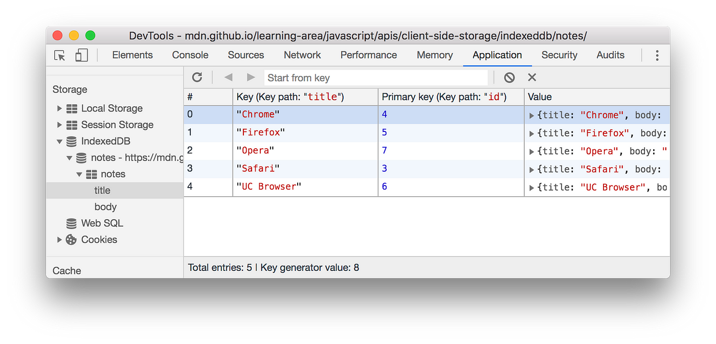
The same-origin policy restricts DB access to the same protocol, host, and port.
| Scope | Control | Example |
|---|---|---|
| Device | OS user, key store | OS login, keychain, disk crypto |
| Browser | Origin, profile | Cookie flags, IDB per origin |
| Tab | Session state | sessionStorage role for API checks |
// set per tab
sessionStorage.setItem("API_KEY", "idb_apikey:nurse:98D1B7");
// read role
const role = (sessionStorage.getItem("API_KEY") || "")
.split(":")[1];
// tiny ACL
const ACL = {
patient: ["read:own"],
nurse: ["read:any","write:notes"],
physician: ["read:any","write:any"]
};
const can = (r,a) => ACL[r]?.includes(a);
// guarded IndexedDB write
if (!can(role, "write:notes"))
throw new Error("forbidden");
const db = await new Promise((res, rej) => {
const req = indexedDB.open("clinic", 1);
req.onupgradeneeded = () =>
req.result.createObjectStore("notes", {
keyPath: "_id"
});
req.onsuccess = () => res(req.result);
req.onerror = () => rej(req.error);
});
const tx = db.transaction("notes", "readwrite");
tx.objectStore("notes").put({ _id, patientId, text });
await tx.done; // or listen to tx.oncomplete
// example keys per role
"idb_apikey:patient:72F3A9"
"idb_apikey:nurse:98D1B7"
"idb_apikey:physician:65A4C2"
// Example: Express middleware
app.use((req, res, next) => {
const token = req.headers.authorization;
// patient, nurse, physician
const role = verifyJWT(token).role;
req.role = role;
next();
});
app.get("/records/:id", (req, res) => {
if (req.role !== "physician")
return res.status(403).send("forbidden");
db.records.findOne({ _id: req.params.id })
.then(r => res.json(r));
});
// API key example
API_KEY = "backend_apikey:physician:65A4C2"
role = API_KEY.split(":")[1]; // physician
Access decisions occur in the backend: not the database.
# Example: MongoDB Atlas IP access list
Project → Network Access → IP Whitelist
Add IP: 203.0.113.15 (office)
Add CIDR: 203.0.113.0/24 (VPN subnet)
// Self-hosted: bind and firewall
net:
bindIp: 127.0.0.1,192.168.10.5
port: 27017
# OS firewall
sudo ufw allow from 192.168.10.0/24 to any port 27017
Only approved network sources can reach the database.
// Example API keys
API_KEY_PATIENT = "mongo_apikey:patient:72F3A9";
API_KEY_NURSE = "mongo_apikey:nurse:98D1B7";
API_KEY_PHYSICIAN = "mongo_apikey:physician:65A4C2";
// Check and enforce
const role = req.get("x-api-key").split(":")[1];
if (role === "nurse") db.notes.updateOne({ patientId }, update);
else if (role === "patient") db.notes.find({ self: true });
| Aspect | Encryption | Access Control |
|---|---|---|
| Pros |
|
|
| Cons |
|
|
// Example split
patients_core → demographics, ID
patients_medical → diagnoses, treatments
patients_billing → invoices, payments
// Example shard keys
hospital_east → patients.region = "East"
hospital_west → patients.region = "West"
hospital_central → patients.region = "Central"
// Example marts
mart_clinical → patient outcomes
mart_billing → payments, reimbursements
mart_staffing → scheduling, hours
Question:
Design a database pipeline from source to dashboard that protects GPS
data.
Audit Goal:
- Detect vulnerabilities
- Verify compliance
- Improve readiness
{
"audit_area": "Access Control",
"finding": "Too many admin users",
"risk": "Privilege misuse",
"recommendation": "Role-based access"
}
Audit Report (Excerpt)
----------------------
✔ Encryption in transit (TLS)
⚠ Weak password policy
⚠ Shared DB credentials
✔ Regular patch updates
Preventive → stops risk
Mitigating → reduces impact
Audit = Mitigating measure
Question:
What security audit steps would you include to
mitigate risk in a farm IoT data pipeline?
| Query Type | Example |
|---|---|
| Keyword Search | “corn yield” |
| Vector Search | “find farms like this one” |
| Result | Semantically similar records, not just identical text |
| Query | Limitation |
|---|---|
| SELECT * FROM farms WHERE crop='corn' | Exact only |
| SELECT * FROM soils WHERE pH BETWEEN 6 AND 7 | Numeric range only |
| Find farms “like” Farm X | Not supported natively |
| Data | Embedding (3D) |
|---|---|
| “Wheat yield in dry soil” | [0.22, 0.45, 0.10] |
| “Corn yield in low rainfall” | [0.21, 0.44, 0.11] |
| “Rice yield in wet soil” | [0.10, 0.30, 0.50] |
| Farm | Vector | Distance |
|---|---|---|
| F1 (Corn) | [0.20, 0.40, 0.15] | 0.02 |
| F2 (Wheat) | [0.25, 0.30, 0.18] | 0.10 |
| F3 (Rice) | [0.15, 0.45, 0.20] | 0.04 |
| Aspect | SQL/NoSQL | Vector DB |
|---|---|---|
| Query Type | Exact | Semantic |
| Data Type | Structured | Unstructured + Numeric |
| Example | WHERE crop='corn' | Farms similar to F1 |
| Result | Identical matches | Similar contexts |
| # | Likely Type | Typical System | Key Value Fit | Graph Fit |
|---|---|---|---|---|
| 1 | Similarity | Vector DB | No | Sometimes |
| 2 | Aggregation | SQL or OLAP | No | Rare |
| 3 | Document or Row | SQL or NoSQL | Yes for id lookup | No |
| 4 | Similarity | Vector DB | No | Sometimes |
| 5 | Aggregation | SQL | No | Rare |
| Name | License | GitHub / Website |
|---|---|---|
| FAISS | Open Source | github.com/facebookresearch/faiss |
| Milvus | Open Source | github.com/milvus-io/milvus |
| Weaviate | Open Source | github.com/weaviate/weaviate |
| Qdrant | Open Source | github.com/qdrant/qdrant |
import numpy as np
import faiss
# Sample farm data (rainfall, soil_pH, yield)
data = np.array([
[0.75, 0.60, 0.82],
[0.80, 0.62, 0.81],
[0.25, 0.30, 0.28],
[0.78, 0.65, 0.85]
], dtype='float32')
# Build index (L2 distance)
index = faiss.IndexFlatL2(3)
index.add(data) # add all farm vectors
# Query: find 3 nearest farms to first one
query = np.array([[0.75, 0.60, 0.82]], dtype='float32')
D, I = index.search(query, k=3)
print(I) # indices of similar farms → [[0 3 1]]
print(D) # similarity distances → [[0.0000 0.0013 0.0025]]
Before:
{"farm":"F1","lat":37.95,"lon":-121.29,"rain":3.4}
After:
{"farm":"F1","gps_enc":"b9a3f1...","rain":3.4}
Before:
{"farm":"F1","rain":"3.4mm","temp":"22C"}
After:
{"farm":"F1","rain_mm":3.4,"temp_c":22.0}
Before:
{"farm":"F1","rain":3.4}
{"farm":"F1","yield":4.8}
After:
{"farm":"F1","rain":3.4,"yield":4.8}
Before:
{"farm":"F1","rain":3.4,"ph":6.3,"yield":4.8}
After:
{"id":"A1","vector":[0.62,0.58,0.73]}
Before:
{"query":"A1"}
After:
{"neighbors":[{"id":"A1","dist":0.0},
{"id":"A2","dist":0.07}]}
Before:
{"farm":"F1","gps":[37.95,-121.29]}
After:
{"farm":"F1","region":"Valley","gps":"hidden"}
{
"pipeline":"secure_farm_data",
"stages":["ingest","curate","vector","serve"],
"security":["encrypt","access","audit"]
}
Before:
{"farm":"F1","rain":3.4,"ph":6.3,"yield":4.8}
After:
{"id":"A1","vector":[0.62,0.58,0.73]}
Before:
{"farm":"F2","rain":2.1,"ph":6.7,"yield":4.2}
After:
{"id":"A2","vector":[0.39,0.71,0.61]}
Before:
{"query":"A1","k":3}
After:
{"neighbors":[
{"id":"A1","dist":0.00},
{"id":"A2","dist":0.07},
{"id":"A3","dist":0.12}
]}
Before:
{"neighbors":[{"id":"A2"},{"id":"A3"}]}
After:
{"neighbors":[
{"id":"A2","region":"Valley","gps":"hidden","dist":0.07},
{"id":"A3","region":"Foothill","gps":"hidden","dist":0.12}
]}
Before:
{"vector":[1.9,-0.4,7.2]}
After:
{"error":"out_of_range","action":"reject"}
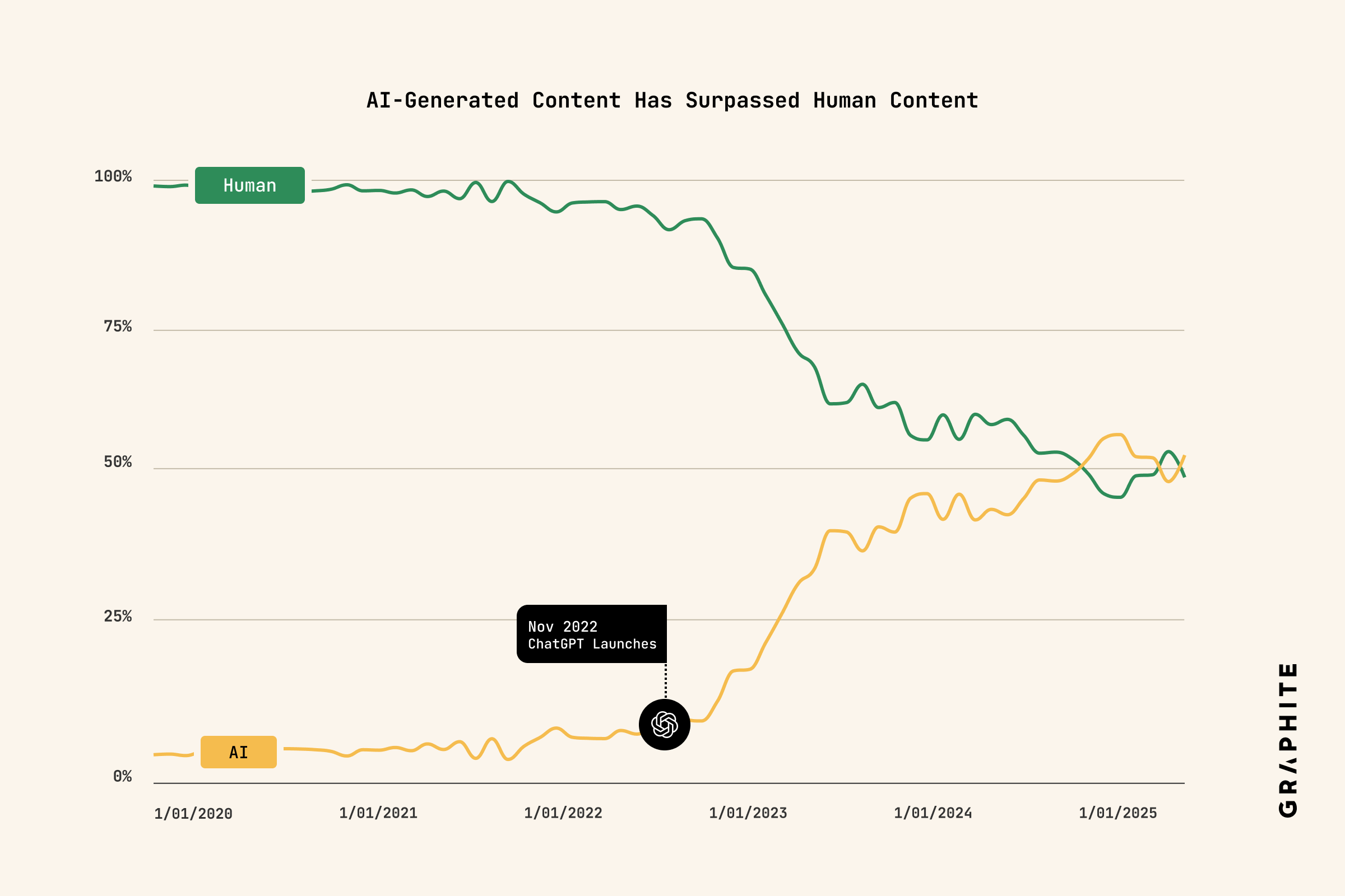

IndexedDB Structure
weatherStore.
// IndexedDB stored record
{
id: 101,
city: "Stockton",
temp: 92,
humidity: 40,
date: "2025-08-01"
}
SQL Table Structure
-- SQL row stored in table
id | city | temp | humidity | date
-----------------------------------------
101 | Stockton | 92 | 40 | 2025-08-01
// IndexedDB Read (weather)
store.get(cityKey); // primary key lookup (B-tree)
store.getAll(); // load all records
SELECT * FROM weather
WHERE city = 'Stockton';
SELECT * FROM weather w
JOIN regions r
ON w.region_id = r.id;
Query fastest to find yesterday’s temperature record?
SELECT * FROM weather
WHERE date = 'yesterday';
-- or with index
SELECT * FROM weather
WHERE date = 'yesterday';
Write an IndexedDB query:
// Load all weather records, then filter and map
store.getAll().onsuccess = (event) => {
const weather = event.target.result; // n records
const hotCities =
weather
.filter(w => w.temp >= 90) // O(n)
.map(w => w.city); // O(n)
// Total time ~ O(n) for n records
};
MongoDB Document
weather.
{
_id: 101,
city: "Stockton",
temp: 92,
hum: 40,
date: "2025-08-01"
}
SQL Row
id | city | temp | hum | date
-----------------------------------
101| Stockton | 92 | 40 | 2025-08-01
insertOne()find()updateOne()deleteOne()
db.weather.find({
temp: { $gte: 90 }
})
SELECT city FROM weather
WHERE temp >= 90;
Fastest way to find all cities with temp ≥ 90?
find() no index)Write a MongoDB query:
// MongoDB MQL
db.weather.find({ city: "Stockton" })
-- SQL
SELECT * FROM weather
WHERE city = 'Stockton';
Redis Hash
weather:101.
KEY: weather:101
FIELDS:
city = "Stockton"
temp = "92"
hum = "40"
date = "2025-08-01"
SQL Row
weather.
id | city | temp | hum | date
-----------------------------------
101| Stockton | 92 | 40 | 2025-08-01
HSET weather hash.HGETALL / HGET.HSET same key.DEL weather:101.
HGETALL weather:101
SELECT * FROM weather
WHERE id = 101;
Fastest way to get yesterday’s weather for id 101?
Task:
HGETALL weather:101
SELECT * FROM weather
WHERE id = 101;
ClickHouse (Daily Aggregates)
weather_daily_city.
-- ClickHouse aggregate row
city | date | avg_temp | max_temp | count
-------------------------------------------------
Stock | 2025-08-01 | 87.2 | 102 | 1440
Row-Store SQL (Raw Readings)
weather_raw.
-- Row-store raw row
city | date | time | temp | hum
----------------------------------------
Stock | 2025-08-01 | 12:00 | 92 | 40
weather_raw.weather_daily_city.
-- ClickHouse (pre-aggregated)
SELECT city, avg_temp
FROM weather_daily_city
WHERE date = '2025-08-01';
-- Row-store (raw)
SELECT city,
AVG(temp) AS avg_temp
FROM weather_raw
WHERE date = '2025-08-01'
GROUP BY city;
Average temperature per city for 3 years of data.
weather_raw (GROUP BY).weather_raw (GROUP BY).weather_daily_city.Task:
-- ClickHouse (aggregate table)
SELECT city,
max_temp
FROM weather_daily_city
WHERE date >= '2025-08-01'
AND date <= '2025-08-31';
-- Row-store (raw table)
SELECT city,
MAX(temp) AS max_temp
FROM weather_raw
WHERE date BETWEEN '2025-08-01'
AND '2025-08-31'
GROUP BY city;
FAISS Index
# vector for a city
[0.12, -0.30, 0.75, ...]
SQL Table with Vectors
weather_vectors.
city | vec
-----------------------
"Stock" | [0.12,-0.30,...]
# FAISS: query q, get top-k
D, I = index.search(q, k)
# I = vector ids for nearest cities
-- SQL pseudo (no vector index)
SELECT city,
distance(vec, :q) AS d
FROM weather_vectors
ORDER BY d
LIMIT 10;
Task: Top 10 similar cities for a weather embedding.
Task:
# FAISS
k = 5
D, I = index.search(q, k)
# I = nearest vector ids
-- SQL pseudo
SELECT id
FROM weather_vectors
ORDER BY distance(vec, :q)
LIMIT 5;

Which change most fundamentally shifted data management after 2000?
Why were pre-2000 systems unable to support today’s data scale?
What made rigid SQL schemas insufficient for modern IoT and mobile apps?
Why did NoSQL architectures become necessary in the 2000s?
Why is IndexedDB considered I/O bound in the browser?
What is the main performance benefit of using a database index?
What isolates IndexedDB data access between different tabs?
Why must IndexedDB CRUD operations often be awaited in JavaScript?
Which ACID property is only partially guaranteed by IndexedDB?
Which scenario is IndexedDB best suited for in practice?
{
"farmId": 101,
"farmName": "Green Valley Farm",
"location": 'Stockton, CA',
crops: ["wheat", "corn", "almonds"],
"areaHectares": 25.5,
"irrigated": True,
"soilType": "loam",
"sensorIds": [1001, 1002,],
"lastInspection": "2025-09-04T10:15:30Z",
"owner": "Alice",
"notes": "North field needs fertilizer",
// pending certification
"certifiedOrganic": "false"
}How many JSON syntax errors can you spot in the snippet on the left?
{
"farmId": "ABC-999",
"farmName": "Green Valley Farm",
"location": "Stockton, CA",
"areaHectares": -12,
"irrigated": "yes",
"soilType": "liquid",
"crops": [],
"sensorCount": 50000,
"lastInspection": "3025-01-01T10:00:00Z",
"ownerId": null,
"averageYieldKg": "high",
"active": "sometimes",
"coordinates": "not available",
"waterUsageLiters": -500,
"notes": "Healthy season expected"
}How many semantic errors can you identify in the JSON on the left?
Which structure best describes a JSON object according to the standard?
What is the defining property of a JSON array?
Which rule about keys in a JSON object is required by the JSON standard?
In JSON, what does the literal null represent?
Why is nesting related fields inside a JSON object often recommended?
Why should JSON objects in distributed systems include a unique id field?
What is the main advantage of using UUIDs as IDs in JSON documents?
Why is ISO 8601 widely used for timestamps in JSON-based APIs?
In a timestamp like 2025-09-04T10:15:30Z, what does the trailing
Z indicate?
map do?
filter do?
reduce?
map operation in IndexedDB?
$group$project$match$sum$matchNoSQL, Key-Value Store, Document Store, Column Store, Graph Database, CAP Theorem, BASE Model, Eventual Consistency, ACID Properties, Strong Consistency, Data Warehouse, Sharding, Replication, Partitioning, Data Mart, Fact, Dimension, Volume, Velocity, Variety, Veracity, Value, Horizontal Scaling, Vertical Scaling, Consistency, Availability, Partition Tolerance, Vector Clock, Schema-less, Indexing, Secondary Index, Primary Key, Neo4j, Compound Key, MapReduce, Aggregation, Query Engine, Query Planner, Execution Plan, CRUD, Insert, Update, Delete, Read, Write Concern, Read Concern, Consistency Level, Consistency, onupgradeneeded, createObjectStore, keyPath, autoIncrement, transaction, objectStore.add, createIndex, Latency, Throughput, Fault Tolerance, Failover, Replica Set, Leader Election, Cluster, Data Center, Geo-Replication, Document Model, BSON, XML Store, Wide Column, Super Column, Column Family, CQL, MQL, Cypher, Graph Traversal, Property Graph, RDF, Triple Store, Relationship, Node, Edge, NoSQL, Index-Free Adjacency, Query Optimization, Materialized View, Denormalization, Data Redundancy, Write Amplification, Compaction, Commit Log, Snapshot, Backup, Restore, Hot Data, Cold Data, Data Lake, Data Warehouse, ETL, ELT, Streaming, Batch Processing,, Transformation, Lambda Architecture, Pub/Sub, Message Queue, Idempotency, Conflict Resolution, Event Sourcing, CQRS, Distributed Cache, In-Memory Database, Time-Series Database, Search Index, Map, Filter, Reduce, Inverted Index, Full-Text Search, Accuracy, Completeness, Consistency, Timeliness, Validity, Uniqueness, Integrity, Usability. Atlas, Compass, Collection, find, updateOne, deleteOne, deleteMany, aggregate, $match, $group, $sort, $limit, $set, $inc, MATCH (alice:Person {name: 'Alice'})-[:FRIEND]->(friend), MATCH (bob:Person {name: 'Bob'})-[:FRIEND]->(friend), MATCH (alice:Person {name: 'Alice'}), MATCH (bob:Person {name: 'Bob'}), $jsonSchema, createCollection, createIndex, IndexedDB, UUID, ObjectId
Course Syllabus – Fall 2025
This course explores managing large volumes of unstructured and evolving data. Emphasis on hands-on labs, projects, and real-world domains (IoT in agriculture, automotive, retail, healthcare). Students contrast modern challenges with traditional SQL concepts.